Transport coefficients from the lattice?

Abstract

The prospects of extracting transport coefficients from euclidean lattice simulations are discussed. Some general comments on the reconstruction of spectral functions using the Maximal Entropy Method are given as well.

1. In field theory transport coefficients are proportional to the slope of appropriate spectral functions at zero frequency and zero spatial momentum (Kubo relation). Examples are the electrical conductivity,

$$\sigma=\frac{1}{6}\frac{\partial}{\partial\omega}\rho_{\rm em}(\omega,{\mathbf{0}})\Big{|}_{\omega=0},$$ (1)

where $\rho_{\rm em}(x,y)=\langle[j_{\rm em}^{i}(x),j_{\rm em}^{i}(y)]\rangle$ is the spectral function associated with the electromagnetic current $j_{\rm em}^{i}=\bar{\psi}\gamma^{i}\psi$, and the shear viscosity,

$$\eta=\frac{1}{20}\frac{\partial}{\partial\omega}\rho_{\pi\pi}(\omega,{\mathbf{0}})\Big{|}_{\omega=0},$$ (2)

where $\rho_{\pi\pi}(x,y)=\langle[\pi_{kl}(x),\pi_{kl}(y)]\rangle$ with $\pi_{kl}$ the traceless part of the spatial energy-momentum tensor.

The euclidean two-point function and the spectral function (both at zero momentum) are related via a dispersion relation and

$$G(\tau)=\int_{0}^{\infty}\frac{d\omega}{2\pi}\,K(\tau,\omega)\rho(\omega),$$ (3)

with the kernel

$$K(\tau,\omega)=e^{\omega\tau}n_{B}(\omega)+e^{-\omega\tau}\left[1+n_{B}(\omega)\right],$$ (4)

where $n_{B}(\omega)=1/[e^{\omega/T}-1]$ is the Bose distribution. The first attempt to compute transport coefficients on the lattice using Eq. (3) was made some time ago by Karsch and Wyld [2], by fitting a three-parameter ansatz for the spectral function to the euclidean lattice data. This approach was pursued more recently in Ref. [3]. A modern way to attack this problem would of course be to use the Maximal Entropy Method [4]. Once the spectral function is reconstructed for all $\omega$, the transport coefficient is in principle determined.

Two obvious questions are: What is the spectral function expected to look like at high temperature? How does the transport coefficient, or in general the low-frequency part of the spectral function, show up in the euclidean correlator?

2. To answer the first question, we calculated the spectral function relevant for the shear viscosity at high temperature in weakly-coupled scalar and nonabelian theories [1]. The results for the scalar theory are sketched in Fig. 1. The contribution at higher frequencies, i.e. $\omega\gtrsim 2m$ where $m$ is the thermal mass, arises from (inverse) decay processes. At large enough $\omega$ the spectral function increases as $\rho_{\pi\pi}(\omega)=(\omega^{4}/96\pi)\left[1+2n_{B}(\omega/2)\right]$. The origin of the contribution at lower frequencies is scattering of fast-moving particles with soft bosons in the plasma. The approximate shape of the spectral function in this region is given by

$$\frac{\rho_{\pi\pi}(\omega)}{T^{4}}\sim\frac{\omega\gamma}{\omega^{2}+4\gamma^{2}}\;\;\;\;\;\;\;\;\;\;\;\;\;\;\;(\omega\ll T),$$ (5)

where $\gamma$ is the thermal damping rate. The particular form in Eq. (5) is due to the presence of poles in the complex energy-plane that pinch the real axis from above and below. The denominator indicates the distance between these so-called pinching poles. The viscosity is determined by the slope at zero frequency and is proportional to $1/\gamma$. A quantitative analytical calculation in this regime is complicated since due to the pinching poles the loop expansion breaks down and all ladder diagrams with uncrossed rungs contribute at leading order in the coupling [5]. In the scalar theory, the low- and the high-frequency contribution match parametrically around the threshold for decay, $\omega=2m$.

Figure 1: Sketch of the spectral function $\rho_{\pi\pi}(\omega)/T^{4}$ versus $\omega$ in a weakly-coupled scalar $\lambda\phi^{4}$ theory (not to scale). The shear viscosity is given by the slope at zero frequency. See the main text for discussion.

A general ansatz describing the low-frequency contribution is

$$\frac{\rho^{\rm low}_{\pi\pi}(x)}{T^{4}}=x\frac{b_{1}+b_{2}x^{2}+b_{3}x^{4}+\ldots}{1+c_{1}x^{2}+c_{2}x^{4}+c_{3}x^{6}+\ldots},$$ (6)

where $x=\omega/T$ and $b_{i}=c_{i}=0$, $i>n$ for given $n$. For gauge theories the overall characteristic shape remains as in Fig. 1 but the dependence on the coupling constant $g^{2}\sim\lambda$ differs somewhat [1].

3. We now address the second question raised in the beginning. At leading order in the coupling constant the euclidean correlator can be computed exactly using Eq. (3), and we find

$$G_{\pi\pi}(\tau)= \frac{a_{1}\pi^{2}T^{5}}{3\sin^{5}u}\Big{\{}(\pi-u)\left[11\cos u+\cos 3u\right]$$ (7)

$$+\,6\sin u+2\sin 3u\Big{\}}+\frac{4a_{2}\pi^{2}}{45}T^{5},$$

with $u=2\pi\tau T$. For the scalar theory $a_{1}=a_{2}=1$, while for an $SU(N_{c}$) theory $a_{1}=6a_{2}=12(N_{c}^{2}-1)$. The $\tau$-dependent terms arise entirely from the high-frequency part of the spectral function. The $\tau$-independent term originates from the low-frequency part. The fact that the low-frequency part of the spectral function leads to a constant term in the euclidean correlator is easily understood. Since for small frequencies $\omega\ll T$ the kernel (4) can be expanded as

$$K(\tau,\omega)=\frac{2T}{\omega}+{\cal O}\left(\frac{\omega}{T}\right),$$ (8)

and the dominating term at small $\omega$ is $\tau$-independent, the low-frequency part of the spectral function corresponds in the euclidean correlator to a constant term proportional to $\int d\omega\,\rho_{\pi\pi}(\omega)/\omega$. This particular constant cannot be easily disentangled from the high-frequency contribution. This is illustrated in Fig. 2, where we plot the analytical result for $G_{\pi\pi}(\tau)$ in the case of $SU(3)$. The tiny difference between the full and the dashed lines is due to the constant term in Eq. (7). Once again, this term originates from the low-frequency part of the spectral function and reflects $\int d\omega\,\rho_{\pi\pi}(\omega)/\omega$, not $\rho_{\pi\pi}(\omega)$ itself. Therefore, we find that $G_{\pi\pi}(\tau)$ is remarkably insensitive to details of $\rho_{\pi\pi}(\omega)$ when $\omega\ll T$ and we conclude that it is extremely difficult to extract transport coefficients in weakly-coupled field theories from the euclidean lattice.

4. The results described above are generic and not specific for the correlators we considered. The fact that the low-frequency part of a spectral function corresponds to a constant term in the euclidean correlator relies solely on the expansion (8). In our opinion this result is a potential problem for the Maximal Entropy Method when the reconstruction of low-frequency parts of spectral functions is attempted. We emphasize that the difficulty is not a numerical one, e.g. due to a finite number of lattice points in the imaginary-time direction. Furthermore, it is easy to see that at finite temperature the presence of pinching poles in correlators of composite operators that are bilinear in the fields is quite common. From general considerations it follows that the effect of pinching poles is a low-frequency contribution as in Eqs. (5, 6) and Fig. 1.

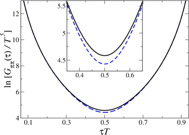
Figure 2: Logarithm of $G_{\pi\pi}(\tau)/T^{5}$ versus $\tau T$ in weakly-coupled $SU(3)$ (Eq. (7), full line). The dashed line is the result without the constant contribution originating from the low-frequency part of the spectral function. The inset shows a blowup around $\tau T=0.5$.

Consider for instance the electromagnetic current-current correlator (or any two-point function of fermion bilinears) in the deconfined quark-gluon plasma. For large frequencies a perturbative calculation gives $\rho_{\rm em}(\omega)\sim\omega^{2}\left[1-2n_{F}(\omega/2)\right]$, where $n_{F}(\omega)=1/[e^{\omega/T}+1]$ is the Fermi distribution and the proportionality factor depends on the number of fermions, colours, etc. For this reason it is customary to present this kind of spectral functions as $\rho_{\rm em}(\omega)/\omega^{2}$. However, due to pinching poles also this spectral function is expected to have a structure at small frequencies as in Eqs. (5, 6) and Fig. 1, where in this case $\gamma$ is the fermion damping rate. For very small frequencies the spectral function can be expanded as

$$\frac{\rho_{\rm em}(\omega)}{T^{2}}=d_{1}\frac{\omega}{T}+d_{3}\left(\frac{\omega}{T}\right)^{3}+d_{5}\left(\frac{\omega}{T}\right)^{5}+\ldots,$$ (9)

where $d_{1}$ is proportional to the electrical conductivity. The coefficients $d_{i}$ are nonzero at finite temperature only and represent repeated scattering of the fast-moving on-shell fermions with soft gauge bosons in the deconfined phase of the high-temperature plasma. Because of this behaviour, $\rho_{\rm em}(\omega)/\omega^{2}$ diverges as $1/\omega$ when $\omega\to 0$. Singular behaviour at very small frequencies of spectral functions of fermion bilinears that are normalized with $1/\omega^{2}$ has indeed been found [6] although the statistical significance of these results is still uncertain.

References

- [1] G. Aarts and J. M. Martínez Resco, JHEP 0204, 053 (2002) [hep-ph/0203177].
- [2] F. Karsch and H. W. Wyld, Phys. Rev. D 35 (1987) 2518.
- [3] A. Nakamura, S. Sakai and K. Amemiya, Nucl. Phys. Proc. Suppl. 53 (1997) 432 [hep-lat/9608052]; A. Nakamura, T. Saito and S. Sakai, ibid. 63 (1998) 424 [hep-lat /9710010]; 106 (2002) 543 [hep-lat/0110177].
- [4] See e.g. M. Asakawa, T. Hatsuda and Y. Nakahara, Prog. Part. Nucl. Phys. 46 (2001) 459 [hep-lat/0011040]; T. Yamazaki et al. [CP-PACS Collaboration], Phys. Rev. D 65 (2002) 014501 [hep-lat/0105030]; F. Karsch et al., Phys. Lett. B 530 (2002) 147 [hep-lat/0110208]; and various contributions to this conference.
- [5] S. Jeon, Phys. Rev. D 52 (1995) 3591 [hep-ph/9409250].
- [6] See e.g. M. Asakawa, T. Hatsuda and Y. Nakahara, hep-lat/0208059.