ITEP-LAT/2002-12
KANAZAWA-02-25
3 September, 2002
Gluon propagators in maximal abelian gauge of $SU(2)$ lattice gauge theory

Abstract

We study propagators of diagonal and off-diagonal gluons in the momentum space in maximal abelian gauge of $SU(2)$ lattice gauge theory. Remaining $U(1)$ degrees of freedom are fixed using Landau gauge. We find substantial difference between the propagator of the diagonal and the off-diagonal gluon in the infrared region. The propagator of the off-diagonal gluon is suppressed in comparison with that of the diagonal gluon at small momenta. In the ultraviolet region both propagators behave as in nonabelian Landau gauge.

1 INTRODUCTION

In lattice numerical studies gauge invariant quantities are usually computed. On the other hand, gauge covariant quantities also provide important information. The well known examples are quark and gluon propagators, requiring complete gauge fixing, monopoles and P-vortices, which study needs only partial gauge fixing. The first lattice calculations of the gluon propagator were performed in Landau gauge [1]. Nowadays these results are significantly improved , also various gauges are used (see e.g. [2]). Maximal abelian gauge (MAG), used to demonstrate the dual super conductor confinement mechanism, is especially interesting. Propagators in this gauge were not explored carefully enough so far. The first such study of propagators in the coordinate space was performed in Ref. [3]. There was no study of propagators in the momentum space. In this paper our aim is to close this gap. We present our results of the high statistics calculation of propagators of the diagonal and the off-diagonal gluon in $SU(2)$ lattice gauge theory in MAG. Complete gauge fixing is achieved by using abelian Landau gauge to fix remaining abelian gauge degrees of freedom.

2 GAUGE FIXING

We use the standard parameterization of $SU(2)$ link matrices, $U_{11}=e^{i\theta}\cos\varphi,\ U_{12}=e^{i\chi}\sin\varphi$. Then gauge fields are defined as follows:

$$A^{1}_{\mu}(x) =\sin\varphi_{\mu}(x)\sin\chi_{\mu}(x),$$ (1)

$$A^{2}_{\mu}(x) =\sin\varphi_{\mu}(x)\cos\chi_{\mu}(x),$$ (2)

$$A^{3}_{\mu}(x) =\cos\varphi_{\mu}(x)\sin\theta_{\mu}(x).$$ (3)

We call $A_{\mu}^{3}(x)$ the diagonal gluon field, and $A_{\mu}^{i}(x),\ i=1,2$ the off-diagonal gluon field.

The maximal abelian gauge condition in a differential form is

$$(\partial_{\mu}\mp iA^{3}_{\mu}(x))A^{\pm}_{\mu}(x)=0;\ A^{\pm}_{\mu}=\frac{1}{\sqrt{2}}(A^{1}_{\mu}\pm iA^{2}_{\mu}).$$

Nonperturbative fixing of this gauge amounts to the minimization of the functional

$$F[A]=\int d^{4}x((A^{1}_{\mu}(x))^{2}+(A^{2}_{\mu}(x))^{2}).$$

In our simulations the Simulated Annealing algorithm [4] with 20 randomly generated gauge copies is employed to minimize the effect of Gribov copies.

After MAG, only $U(1)$ degrees of freedom remain unfixed. We fix them using $U(1)$ Landau gauge. The differential lattice gauge condition we are using is

$$\Delta_{\mu}\sin\theta_{\mu}(x)=0.$$ (4)

This condition implies that the diagonal field $A_{\mu}^{3}$ is not transversal at a finite lattice spacing. Another gauge condition $\Delta_{\mu}A^{3}_{\mu}=0$ is not considered here and will be discussed elsewhere [5]. Condition (4) is equivalent to the maximization of the functional

$$F[\theta]=\sum_{x,\mu}\cos\theta_{\mu}(x),$$

using only $U(1)$ gauge transformations. A local maximization algorithm with 30 random gauge copies is used to accomplish this task. As the ”stop criterion” for the algorithm we use

$$\frac{F[\theta]_{new}-F[\theta]_{old}}{F[\theta]_{new}}<\varepsilon=10^{-8}.$$ (5)

3 PROPAGATORS

We calculate the diagonal propagator

$$D_{\mu\nu}^{diag}(p)=D^{33}_{\mu\nu}(p)=\langle{\cal A}^{3}_{\mu}(k){\cal A}^{3}_{\nu}(-k)\rangle,$$ (6)

and the off-diagonal propagator

$$D_{\mu\nu}^{offdiag}(p)=D^{11}_{\mu\nu}(p)=D^{22}_{\mu\nu}(p)=\\ \langle{\cal A}^{1,2}_{\mu}(k){\cal A}^{1,2}_{\nu}(-k)\rangle,$$ (7)

where Fourier transform ${\cal A}_{\mu}^{i}(k)$ is defined as

$${\cal A}_{\mu}^{i}(k)=\frac{1}{\sqrt{L^{4}}}\sum_{x}e^{-ik_{\nu}x_{\nu}-\frac{i}{2}k_{\mu}}A_{\mu}^{i}(x),$$

$$k_{\mu}=\frac{2\pi n_{\mu}}{aL_{\mu}},n_{\mu}=0,...,L_{\mu}-1.$$

The physical lattice momenta $p$ are related to $k$ as follows:

$$p_{\mu}=\frac{2}{a}\sin{\frac{ak_{\mu}}{2}}.$$

Since both diagonal and off-diagonal fields are not transversal the general structure of diagonal and off-diagonal propagators is

$$D_{\mu\nu}(p)=(\delta_{\mu\nu}-\frac{p_{\mu}p_{\nu}}{p^{2}})D^{t}(p^{2})+\frac{p_{\mu}p_{\nu}}{p^{2}}D^{l}(p^{2}).$$ (8)

Thus we have four structure functions $D^{t,l}_{diag,offdiag}$, which are really not independent. Note that in nonabelian Landau gauge, $\partial_{\mu}A_{\mu}^{a}\tau^{a}=0$, there would be only one formfactor:

$$\langle{\cal A}_{\mu}^{a}(p){\cal A}_{\nu}^{b}(-p)\rangle=\delta^{ab}(\delta_{\mu\nu}-\frac{p_{\mu}p_{\nu}}{p^{2}})D(p^{2}).$$

4 NUMERICAL RESULTS

To calculate propagators the lattice with $L=24$ (138 configurations) at $\beta=2.40$ were simulated. The lattice spacing is $(1.66~{}\text{GeV})^{-1}$ at this $\beta$.

The behavior of transversal parts of propagators in the ultraviolet region is the same as in nonabelian Landau gauge as our gauge corresponds to that gauge in the limit of large momenta. Both gluons are well described by the perturbative formula $D^{t}_{diag,offdiag}(p^{2})=\frac{Z_{diag,offdiag}}{p^{2}}$, see Fig. 1. The longitudinal part $p^{2}D^{l}_{offdiag}(p^{2})$ tends to zero as $p^{2}$ tends to infinity. And $p^{2}D^{l}_{diag}(p^{2})$ is small in comparison with other structure functions (see inset in Fig. 1). It increases linearly with increasing $p^{2}$. Similar result was obtained in [6] for the longitudinal part of the photon propagator in 3D compact QED when gauge condition was chosen allowing nonzero longitudinal part at the finite lattice spacing as in our case. Indications that the longitudinal part tends to zero in the continuum limit were found in [6].

The sharp increase of $p^{2}D^{l}_{diag}(p^{2})$ at low momenta seems to be related to imprecise $U(1)$ Landau gauge fixing. We repeated computations on our smaller $16^{4}$ lattices (300 gauge field configurations) with reinforced condition (5): $\varepsilon$ decreased down to $10^{-10}$. We found that $p^{2}D^{l}_{diag}(p^{2})\rightarrow 0,\ p^{2}\rightarrow 0$, [5].

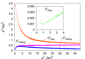
Figure 1: Formfactors of the diagonal and the off-diagonal gluon. The rescaled inset shows $p^{2}D^{l}_{diag}$ with the same axes as in the main plot.

In IR region one can see a very strong suppression of $D^{t}_{offdiag}(p^{2})$ in comparison with $D^{t}_{diag}(p^{2})$ demonstrating the essence of the Abelian dominance [7], Fig.1. At the same time $D^{l}_{offdiag}(p^{2})$ approaches $D^{t}_{offdiag}(p^{2})$ at $p<1.5~{}\text{GeV}$. The off-diagonal propagator thus becomes:

$$D_{\mu\nu}^{offdiag}(p)=\frac{\delta_{\mu\nu}}{p^{2}+m^{2}_{off}(p^{2})}.$$ (9)

Fit to this form at $p<1.5~{}\text{GeV}$ with $\chi^{2}/N_{dof}=1.76$ gives $m_{off}=1.06(1)~{}\text{GeV}$.

In the range $p<1.5~{}\text{GeV}$ the best fit ($\chi^{2}/N_{dof}=0.51$) to $D^{t}_{diag}(p^{2})$ is given by the formula

$$D^{t}_{diag}(p^{2})=\frac{Z\ m_{diag}^{2\alpha}}{(p^{2}+m^{2}_{diag})^{1+\alpha}}.$$ (10)

We obtain $\alpha=0.80(1),\ m_{diag}=0.63(1)~{}\text{GeV}$. This shows that behavior of $D^{t}_{diag}(p^{2})$ in the infrared region is qualitatively similar to that of the propagator in nonabelian Landau gauge [2].

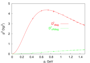
Figure 2: Lattice data fitted by Eq. 10 for the $D^{t}_{diag}(p^{2})$ and by Eq. 9 for $D^{t}_{offdiag}(p^{2})$.

5 CONCLUSIONS AND OUTLOOK

Our results clearly show that off-diagonal gluons are suppressed at low momenta thus providing the explanation of the Abelian dominance established in numerical studies of MAG. Effects of the finite volume and incomplete gauge fixing should be further investigated.

References

[1]
J. E. Mandula and M. Ogilvie,
Phys. Lett. B 185 (1987) 127.
[2]
F. D. Bonnet, P. O. Bowman, D. B. Leinweber, A. G. Williams and J. M Zanotti,
Phys. Rev. D 64 (2001) 034501.
C. Alexandrou, P. de Forcrand and E. Follana,
Phys. Rev. D 63 (2001) 094504.
[3]
K. Amemiya and H. Suganuma,
Phys. Rev. D 60 (1999) 114509.
[4]
G. S. Bali, V. Bornyakov, M. Muller-Preussker and K. Schilling,
Phys. Rev. D 54 (1996) 2863.
[5]
V. G. Bornyakov, S. M. Morozov, M. I. Polikarpov, to be published.
[6]
M. N. Chernodub, E. M. Ilgenfritz and A. Schiller,
Phys. Rev. Lett. 88 (2002) 231601;
M. N. Chernodub, E. M. Ilgenfritz and A. Schiller,
arXiv:hep-lat/0208013.
[7]
T. Suzuki and I. Yotsuyanagi,
Phys. Rev. D 42 (1990) 4257.