Simulating non-commutative field theory

Abstract

Non-commutative (NC) field theories can be mapped onto twisted matrix models. This mapping enables their Monte Carlo simulation, where the large $N$ limit of the matrix models describes the continuum limit of NC field theory. First we present numeric results for 2d NC gauge theory of rank 1, which turns out to be renormalizable. The area law for the Wilson loop holds at small area, but at large area we observe a rotating phase, which corresponds to an Aharonov-Bohm effect. Next we investigate the NC $\phi^{4}$ model in $d=3$ and explore its phase diagram. Our results agree with a conjecture by Gubser and Sondhi in $d=4$, who predicted that the ordered regime splits into a uniform phase and a phase dominated by stripe patterns.

1 INTRODUCTION

In the recent years there has been tremendous activity in the research of field theories on NC spaces. One field of application of such theories is the quantum Hall effect [1]. The boom of interest, however, was triggered by the observation that string and M theory at low energy correspond to NC field theories, see e.g. Ref. [2].

The NC space is characterized by the non-commutativity of some of its coordinates. Here we are concerned with the case where only two coordinates do not commute,

$$[\hat{x}_{\mu},\hat{x}_{\nu}]=i\theta\epsilon_{\mu\nu}\ .$$ (1)

For a review of field theory on NC spaces (“NC field theory”), see Ref. [3]. The non-commutativity yields non-locality in a range of $O(\sqrt{\theta})$. This property implies conceptual problems, but there is also hope that it might provide the crucial link to string theory or quantum gravity. From the technical point of view, it makes the perturbative renormalization even harder than in commutative field theory, because a new type of singularity occurs, which is UV and IR at the same time. Heuristically this can be understood immediately from relation (1) along with Heisenberg’s uncertainty relation. So far, there is no systematic machine for absorbing this kind of mixed UV/IR divergences.

2 GAUGE THEORY ON A NC PLANE

In particular, the NC rank 1 gauge action can be written in a form which looks similar to the familiar (commutative) case,

$$S[A]=\frac{1}{4}\int d^{d}x\,{\rm Tr}(F_{\mu\nu}\star F_{\mu\nu})$$ (2)

$$F_{\mu\nu}=\partial_{\mu}A_{\nu}-\partial_{\nu}A_{\mu}+ig(A_{\mu}\star A_{\nu}-A_{\nu}\star A_{\mu})\ ,$$

where the fields are multiplied by the star product

$$f(x)\star g(x)=e^{\frac{1}{2}i\theta\epsilon_{\mu\nu}\frac{\partial}{\partial x_{\mu}}\frac{\partial}{\partial y_{\nu}}}f(x)g(y)|_{x=y}.$$ (3)

This action is star gauge invariant. Also lattice formulations exist, but they can hardly be simulated: one would need star unitary link variables, construct a measure for them etc.

In 1999 Ishibashi et al. observed [4] that NC $U(n)$ gauge theories can be mapped onto specific versions of the twisted Eguchi-Kawai model (TEK) [5], which has the action

$$S_{TEK}[U]=-N\beta\sum_{\mu\neq\nu}Z_{\mu\nu}\,{\rm Tr}(U_{\mu}U_{\nu}U_{\mu}^{\dagger}U_{\nu}^{\dagger})\ ,$$ (4)

$$Z_{\mu\nu}=e^{2\pi ik/L}=Z_{\nu\mu}^{*}\ \ (\mu\!<\!\nu,\,k\in\mathbb{Z},\,L=N^{2/d})\,.$$

Since this system lives on one point there is only one $N\times N$ link variable in each direction. The factor $Z_{\mu\nu}$ is the twist. This mapping is based on Morita equivalence (an exact equivalence of the corresponding algebras) in the large $N$ limit [4], and on discrete Morita equivalence at finite $N$, which corresponds to NC gauge theory on the lattice [6]. The equivalence holds if we choose

$$k=\frac{N+1}{2}\ ,\quad{\rm and~{}it~{}implies}\quad\theta=\frac{1}{\pi}Na^{2}\ ,$$ (5)

where $N$ must be odd, and $a$ is the lattice spacing in the NC space. Also the Wilson loops, which are defined in the TEK in the obvious way (see below) are mapped onto the Wilson loops in NC gauge theory.

This provides a non-perturbative access to NC gauge theory. The problems with the direct NC lattice formulation are all circumvented by this mapping onto a matrix model; hence this is a real counter example to the “no-free-lunch theorem”.

Here we are interested in pure NC $U(1)$ gauge theory in $d=2$ and we summarize our numeric results of Ref. [7]. For analytical work on this model, see in particular Ref. [8].

Due to Eguchi-Kawai equivalence, the large $N$ limit of the TEK at fixed $\beta$ coincides with the planar large $N$ limit of commutative gauge theory, which has been solved analytically [9]. In that case the Wilson loop obeys an exact area law,

$$\langle W(I\times J)\rangle = e^{-\kappa(\beta)IJ}$$ (6)

$$\kappa(\beta) = -\ln(1-\frac{1}{4\beta})\quad{\rm at}\quad\beta\geq\frac{1}{2}\ .$$

From that framework we adapt the “physical area” $a^{2}IJ$, where $a=\sqrt{\kappa}$. However, for our purposes it is crucial to take the double scaling limit, which keeps $Na^{2}\simeq N/\beta$ constant, so that the corresponding NC parameter $\theta$ remains finite in the large $N$ limit, c.f. eq. (5).

This is different from the planar large $N$ limit; the latter would lead to the Gross-Witten solution, in agreement with the well-known equivalence of $\theta\to\infty$ and commutative gauge theory in the planar large $N$ limit.

The 2d TEK was simulated before [11], but not with the parameters required here. Thanks to a trick introduced in Ref. [10] we could apply a heat bath algorithm.

We focus on the square-shaped Wilson loop,

$$W_{12}(I\times I) = \frac{1}{N}Z_{12}^{I^{2}}\,{\rm Tr}(U_{\mu}^{I}U_{\nu}^{I}U_{\mu}^{\dagger\,I}U_{\nu}^{\dagger\,I})$$ (7)

$$= W_{21}^{*}(I\times I)\ .$$

Note that $W(I):=\langle W_{12}(I\times I)\rangle$ is complex because of the twist. In Fig. 1 we show its behavior in polar coordinates at $N/\beta=32$. We see that a double scaling limit does manifestly exist. Since it corresponds to the continuum limit of 2d NC rank 1 gauge theory, we conclude that its Wilson loop is non-perturbatively renormalizable. At small area (with respect to $O(\theta)$) it is practically real and follows the Gross-Witten area law of eq. (6). Beyond that regime $|W(I)|$ does not decay any more, but the phase grows linearly in the area.

Figure 1: The polar coordinates of the complex Wilson loop $W(I)$ plotted against the physical area $A=a^{2}I^{2}$. At small areas it follows the Gross-Witten area law (solid line). At larger areas the absolute value does not decay any more, but the phase increases linearly.

Fig. 2 shows the asymptotic linear behavior of the phase $\phi$ at different values of $N/\beta\simeq\pi\theta$. In the large area regime, we observe the simple relation

$$\phi=A/\theta\ ,\qquad(A=(aI)^{2}={\rm physical~{}area})$$ (8)

to a very high accuracy. We checked that it holds more generally for rectangular Wilson loops. Hence we can identify this law with the Aharonov-Bohm effect, if we formally introduce a constant magnetic field

$$B=1/\theta$$ (9)

across the plane. In fact, this corresponds exactly to the relation used by Seiberg and Witten when they mapped open strings in a constant gauge background onto NC gauge theory [2]. Moreover, the very same relation was used in the description of the quantum Hall effect, where an electron in a layer was projected to the lowest Landau level [1]. Here we recover this law as a dynamical effect.

Figure 2: The phase of the Wilson loop $W(I)$ at $N=125$ for various values of $N/\beta$, corresponding to different values of $\theta$. At large areas $A>O(\theta)$ the phase $\phi$ agrees with the formula $\phi=A/\theta$, which is shown by straight lines.

We fix again $N/\beta=32$, and we consider now the connected Wilson 2-point function

$$G_{2}^{(W)}=\langle W_{\mu\nu}(I\times I)W_{\nu\mu}(I\times I)\rangle_{c}\in\mathbb{R}\ .$$ (10)

After a wave function renormalization $G_{2}^{(W)}\to\beta^{-0.6}G_{2}^{(W)}$ we observe also here a double scaling regime, see Fig. 3 (on top).

Finally we consider the Polyakov lines

$$P_{\mu}(I)={\rm Tr}(U_{\mu}^{I})\,,\ P_{-\mu}(I)={\rm Tr}(U_{\mu}^{\dagger\,I})\ .$$ (11)

Note that $\langle P_{\mu}(I)\rangle=0$ due to the phase symmetry (which corresponds to translation invariance), but the Polyakov multi-point functions are sensible observables. Fig. 3 (below) shows that also the Polyakov 2-point function

$$G_{2}^{(P)}(I)=\langle P_{\mu}(I)P_{-\mu}(I)\rangle$$ (12)

has a double scaling regime, if we apply the same wave function renormalization again, $G_{2}^{(P)}\to\beta^{-0.6}G_{2}^{(P)}$.

Figure 3: The Wilson 2-point function $G_{2}^{(W)}$ (on top) and the Polyakov 2-point function $G_{2}^{(P)}$ (below), at $N=195$. After performing the same wave function renormalization we find a double scaling regime for each of the 2-point functions.

3 THE NC $\phi^{4}$ MODEL IN $d=3$

We now summarize our ongoing work on the NC $\phi^{4}$ model in $d=3$ [12]. We investigate the phase diagram and compare our observations in particular with a conjecture by Gubser and Sondhi, which was obtained in $d=4$ by a Hartree–type approximation [13]. They studied the phase–diagram in the $m^{2}/\Lambda^{2}$–$\theta\Lambda^{2}$ plane for fixed coupling $\lambda$, where $\Lambda$ is a momentum cut–off. The conjecture can be summarized as follows:

• For small $\theta$ there is an Ising type phase transition between a disordered and uniformly ordered phase.

• For large enough $\theta$ this transition changes its nature, due to UV/IR effects. This phase transition is driven by a mode of the scalar field with non–vanishing momentum, leading to a non–uniformly ordered or striped phase. This phase transition is first order in the regularized theory.

• The theory is renormalizable within the one–loop self–consistent Hartree–type approximation and the first order phase transition turns into second order in the continuum limit.

The action of the NC $\lambda\phi^{4}$ theory reads

$$S=\int d^{d}x\left[\frac{1}{2}\partial_{\mu}\phi\,\partial_{\mu}\phi+\frac{m^{2}}{2}\phi^{2}+\frac{\lambda}{4}\phi^{\star 4}\right]\,,$$ (13)

where the interaction term is a star–product of four scalar fields. We study this model in $d\!=\!3$, and we exclude the time direction from non–commutativity. The spatial coordinates satisfy eq.  (1).

A lattice version of this action can be constructed, but as in Section 2 we map the system on a dimensionally reduced model to enable Monte–Carlo simulations. This mapping was already carried out in Ref. [6]. In our case the scalar field $\phi(\vec{x},t)$ defined on a $N^{2}T$ lattice is mapped on $N\times N$ Hermitian matrices $\hat{\phi}(t)$. Their action takes the form

$$S=\textrm{Tr}\sum_{t=1}^{T}\biggl{[}\frac{1}{2}\sum_{\mu}\left(\Gamma_{\mu}\hat{\phi}(t)\,\Gamma_{\mu}^{\dagger}-\hat{\phi}(t)\right)^{2}$$ (14)

$$\hskip 5.69046pt+\frac{1}{2}\left(\hat{\phi}(t+1)-\hat{\phi}(t)\right)^{2}+\frac{m^{2}}{2}\hat{\phi}^{2}(t)+\frac{\lambda}{4}\hat{\phi}^{4}(t)\biggl{]}\,.$$

There are two kinetic terms according to the two underlying geometries. The matrices $\Gamma_{\mu}$ are called ’twist eaters’ and act here as shift operators. They are defined by the relation

$$\Gamma_{\mu}\Gamma_{\nu}=Z^{*}_{\mu\nu}\Gamma_{\nu}\Gamma_{\mu}\,,$$ (15)

where $Z_{\mu\nu}$ is the twist already introduced in Section 2. Again we have to use odd values of $N$.

For this action we study the phase diagram, but in contrast to Gubser and Sondhi we consider the $m^{2}$–$\lambda$ plane at fixed $\theta$. By analogy we expect a striped phase for large enough $\lambda$.

Our results for $N=15\dots 45$ are summarized in the phase diagram in Fig. 4.

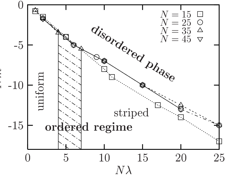
Figure 4: The phase diagram of the 3d NC $\phi^{4}$ theory. The connected points show the separation line between disordered and ordered regime, and the hatched region marks the transition between uniformly ordered and striped phase at $N=35$.

So far we have been able to identify the separation line between ordered regime and disordered phase and we observe a large $N$ scaling. This separation is shown by the points connected with lines. The vertical lines indicate the transition region between uniformly ordered and striped phase at $N=35$. For $N<35$ we find the transition between the two ordered regimes at larger values of $N\lambda$. Below we discuss the procedure that led us to this phase diagram.

We use the momentum dependent order parameter $\langle M(k)\rangle$, where

$$M(k):=\frac{1}{NT}\,\max_{|\vec{p}|=k}\,\bigl{|}\,\sum_{t}\tilde{\phi}(\vec{p},t)\,\bigl{|}\ ,$$ (16)

and $\tilde{\phi}(\vec{p},t)$ is the spatial Fourier transform of $\phi(\vec{x},t)$  . In particular $\langle M(0)\rangle$ reduces to the standard order parameter for the spontaneous breakdown of a $Z_{2}$ symmetry. To find the separation line between ordered and disordered phase, we decreased $m^{2}$ at constant values of $\lambda$, starting in the disordered phase. Two examples at $N=35$ are shown in Fig. 5

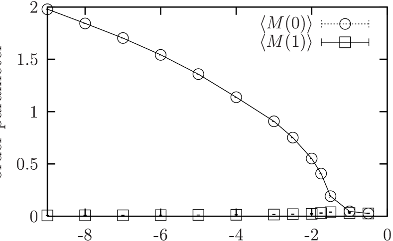
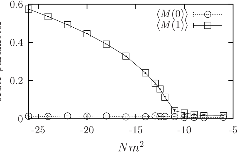
Figure 5: The momentum dependent order parameter against $Nm^{2}$. Above we fixed $N\lambda=2$, which leads to a uniformly ordered phase, and below at $N\lambda=20$ leading to a striped phase.

In these plots we show the standard order parameter $\langle M(0)\rangle$ and the staggered order parameter $\langle M(1)\rangle$. In the upper plot of Fig. 5 only $\langle M(0)\rangle$ is non–trivial below some value of $m^{2}<0$. Therefore we are in the uniformly ordered phase. In the lower plot of Fig. 5, $\langle M(0)\rangle$ practically vanishes for all $m^{2}$, but $\langle M(1)\rangle$ is non–zero, indicating a striped phase. Such measurements allow us to identify the separation region between uniformly ordered and striped phase.

To localize the separation line between ordered and disordered phase we computed the connected part of the two–point function of $M(k)$. This function has a peak at the phase transition. Fig. 6 illustrates some examples for these measurements.

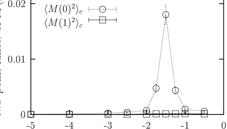
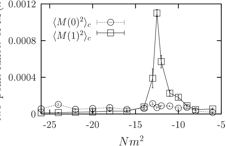
Figure 6: The two–point function of the quantity $M(k)$, defined in eq. (16), against $Nm^{2}$ at $N\lambda=2$ (above) and at $N\lambda=20$ (below).

In Fig. 7 we show some snapshots of configurations $\phi(\vec{x},t)$ at $N=35$. The dotted areas mark the regions where $\phi>0$, and the blank areas represent $\phi<0$. At $N\lambda=2$ and for small $|Nm^{2}|$ (Fig. 7a) we find such areas scattered all over the volume, and at $Nm^{2}\ll 0$ (Fig. 7b) $\phi(\vec{x},t)$ is either positive or negative for all $x$, as one expects for an Ising type phase. At $N\lambda=20$ we also find a disordered phase (Fig. 7c), but for $Nm^{2}\ll 0$ the uniformly ordered phase is replaced by a striped phase (Fig. 7d).

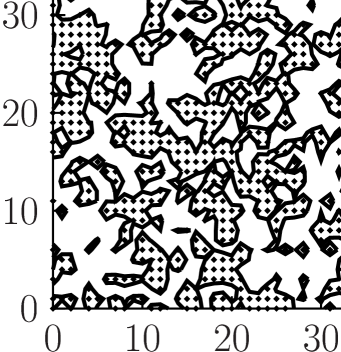
(a) $Nm^{2}=-0.5$

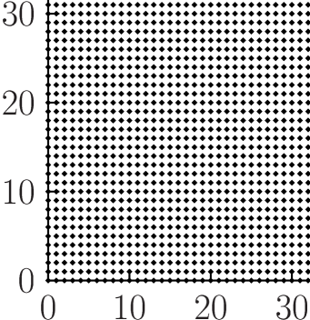
(b) $Nm^{2}=-8$

$N\lambda=2$

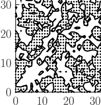
(c) $Nm^{2}=-6$

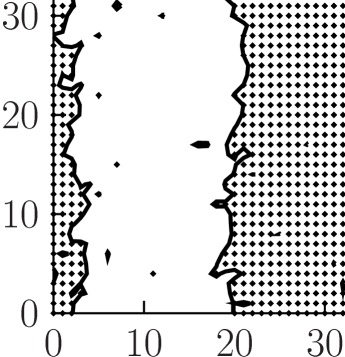
(d) $Nm^{2}=-26$

$N\lambda=20$

Figure 7: Snapshots of single configurations $\phi(\vec{x},t)$ at a certain time $t$, for $N=35$.

4 CONCLUSIONS

We presented numeric results for NC field theory, which could be obtained through the mapping onto twisted matrix models.

In the first part we summarized the results of Ref. [7]. Specific types of the TEK correspond to 2d NC $U(1)$ gauge theory on the lattice. We approached the large $N$ limit so that the non-commutativity parameter $\theta$ is kept constant (double scaling limit). This describes the continuum limit of NC gauge theory. We found finite limits for the 1- and 2-point Wilson loop, as well as the 2-point Polyakov line, which confirms that this model is non-perturbatively renormalizable. This is the first evidence for the non-perturbative renormalizability of a NC field theory.

At small areas, the Wilson loop follows an area law as in the (commutative) planar theory. At larger areas it deviates and reveals a new double scaling limit. This is a manifestation of non-perturbative UV/IR mixing. In that regime, the phase of the Wilson loop is given simply by the area divided by $\theta$. This corresponds to an Aharonov-Bohm effect if we identify $\theta$ with a magnetic field $B=1/\theta$, as it is also done in the solid state [1] and string [2] literature.

We further studied the phase diagram of a 3d NC $\phi^{4}$ theory [12]. The separation line between ordered and disordered phase is localized and we observe large $N$ scaling. In agreement with the qualitative conjecture in Ref. [13], the ordered regime splits into a uniform and a striped phase.

Acknowledgment: We thank A. Barresi, H. Dorn, Ph. de Forcrand and R. Szabo for useful comments.

References

- [1] S. Girvin, A. MacDonald and P. Platzman, Phys. Rev. B33 (1986) 2481.
- [2] N. Seiberg and E. Witten, JHEP 09 (1999) 032.
- [3] M. Douglas and N. Nekrasov, Rev. Mod. Phys. 73 (2002) 977.
- [4] N. Ishibashi, S. Iso, H. Kawai and Y. Kitazawa, Nucl. Phys. B573 (2000) 573.
- [5] A. González-Arroyo and M. Okawa, Phys. Lett. 120B (1983) 174; Phys. Rev. D27 (1983) 2397.
- [6] J. Ambjørn, Y. Makeenko, J. Nishimura and R. Szabo, JHEP 9911 (1999) 029; Phys. Lett. B480 (2000) 399; JHEP 0005 (2000) 023.
- [7] W. Bietenholz, F. Hofheinz and J. Nishimura, hep-th/0203151.
- [8] L. Paniak and R. Szabo, hep-th/0203166.
- [9] D. Gross and E. Witten, Phys. Rev. D21 (1980) 446.
- [10] K. Fabricius and O. Haan, Phys. Lett. 143B (1984) 459.
- [11] K. Fabricius and O. Haan, Phys. Lett. 131B (1983) 399. T. Nakajima and J. Nishimura, Nucl. Phys. B528 (1998) 355. S. Profumo and E. Vicari, JHEP 0205 (2002) 014.
- [12] W. Bietenholz, F. Hofheinz and J. Nishimura, in preparation.
- [13] S. Gubser and S. Sondhi, Nucl. Phys. B605 (2001) 395.