TRINLAT-02/02
QCD on $2+2$ anisotropic lattices

Abstract

We discuss the implementation of QCD on $2+2$ anisotropic lattices. Technical details regarding the choice of the action as well as perturbative and non-perturbative improvement are analyzed. The physical applications of the program are presented.

1 Introduction: Why $2+2$?

QCD on $3+1$ anisotropic lattices [1] has recently proved to be a successful tool for non-perturbative investigation of various interesting physical phenomema (glueball spectrum, $b\bar{b}$ states, gluon strings, spectral density). Although the method is successful for processes where the hadronic final state is static in the center of mass frame, it is less suited to processes where the hadron momentum in the final state is non-negligible compared to its mass. In such cases independent fine space directions for each momentum degree of freedom are needed to describe the system, increasing dramatically the computational cost and the difficulties linked with tuning the parameters. However, there exist some interesting physical phenomena, e.g. $B\!\rightarrow\!K^{*}\,\gamma$, $B\!\rightarrow\!\pi\,l\,\nu$ and $B\!\rightarrow\!\rho\,l\,\nu$, where the final hadron state is either emitted only or strongly peaked at a momentum roughly equal to its mass. Although such systems have been investigated in the $3+1$ case [2], a $2+2$ lattice discretization could allow some improvement in the comparison with experimental data, keeping the “technical” costs at bay. Study of other high-momentum form factors could also benefit from such a program.

2 Setting the Framework: Pure $SU(N_{c})$

Starting from the simple $1\times 1$ plaquette action

$$S_{\rm gluon}=\beta\sum_{x,\mu,\nu}\left(1-\frac{1}{2N_{c}}{c_{\mu\nu}}\,{\rm Re}\,{\rm Tr}\,{P_{\mu\nu}}(x)\right),$$

where the coefficients $c_{\mu\nu}$ must be fixed, either non-perturbatively [3] or perturbatively [4], imposing the recovery of Lorentz invariance in the continuum limit. In the non-perturbative case the coefficients are fixed to restore rotational invariance for, say, the static interquark potential. In lattice perturbation theory the tree level terms are fixed by the naive recovery of the Yang-Mills lagrangian, while higher order corrections in powers of $g^{2}$ will be fixed by the symmetries of the renormalized propagator. The $c_{\mu\nu}$ in lattice perturbation theory are defined as

$$c_{\mu\nu}=\left\{\begin{array}[]{lll}\xi^{2}(1+c_{f}^{(1)}g^{2}+O(g^{4}))&\,\mbox{f-f};\\ 1+\eta^{(1)}g^{2}+O(g^{4})&\,\mbox{c-f};\\ \frac{1}{\xi^{2}}(1+c_{c}^{(1)}g^{2}+O(g^{4}))&\,\mbox{c-c}\end{array}\right.$$ (1)

where $\xi=a_{c}/a_{f}$ is the asymmetry ratio while $c_{f}^{(1)}$, $\eta^{(1)}$ and $c_{c}^{(1)}$ are the coefficients for the fine-fine, fine-coarse and coarse-coarse directions.

Applying lattice perturbative calculations also permits a study of the renormalizability of the theory, important not only for its own sake but also for the extraction of physical matrix elements in the decay processes. The hypercubic physical volume $V$ is fixed and an ultraviolet cutoff, bigger in the $z,\,t$ directions $\lambda_{f}=\xi\lambda_{c}$, is imposed such that $V=L_{c}^{2}L_{f}^{2}\xi^{2}a^{4}$ where $L_{f}=\xi L_{c}$ are the number of sites in the fine and coarse directions. The physical limits are then: $L_{c,f}\!\rightarrow\!\infty$ and $a\!\rightarrow\!0$ keeping $\xi$ fixed. The aim is to make contact with “symmetric” physics, so the procedure is to relate the anisotropic lattice regularization to an asymmetric continuum regularization and from there to a standard continuum regularization. The procedure is general and holds for any anisotropy, including 3+1.

3 Perturbative vs. Non-Perturbative

To perform a perturbative renormalization of the theory the different pieces of asymmetric lattice perturbation theory must be established. Following the symmetric case, the action for the gauge fixing, Faddeev-Popov and measure terms are determined. It will be a general property of Feynman rules not to carry, at tree level, explicit dependence from the asymmetry, where a continuum analogue exists. The only difference resides in the Brillouin zones. On the other hand, at the 1-loop level Lorentz invariance will be broken. Corrections given by the 1-loop $c_{\mu\nu}$ in Eq.(1) are needed to restore it. Moreover, a renormalization procedure must be chosen. In analogy with the symmetric case, PBC are kept and BPHZ with a massive gluon propagator as an intermediate infrared regulator is chosen. Contact with continuum theory is straightforward.

Feynman rules are better calculated in terms of dimensionless quantities

$$\phi_{\mu}(n) = \phi^{b}_{\mu}(n)T^{b}\rightarrow a[\xi]\,gA^{b}_{\mu}(x)T^{b}$$

$$\sum_{n} \rightarrow \frac{1}{\xi^{2}a^{4}}\sum_{x}$$ (2)

where the factor $[\xi]$ will be included according to the value of $\mu$. In this way the pure gauge term reads in the continuum limit as

$$S = \frac{1}{4}\sum_{n}c_{\mu\nu}{\hat{F}^{b}_{\mu\nu}}(n){\hat{F}^{b}_{\mu\nu}}(n)+{\cal O}$$ (3)

$$= \frac{1}{4}\sum_{x}{F^{b}_{\mu\nu}}(x){F^{b}_{\mu\nu}}(x)+O(a^{2})$$

where $\cal O$ is an irrelevant operator and

$$\hat{F}_{\mu\nu} = \hat{\partial}^{R}_{\mu}\phi_{\nu}-\hat{\partial}^{R}_{\nu}\phi_{\mu}+ig[\phi_{\mu},\phi_{\nu}]$$

$$F_{\mu\nu} = \partial^{R}_{\mu}A_{\nu}-\partial^{R}_{\nu}A_{\mu}+ig[A_{\mu},A_{\nu}]$$

$$\partial^{R}_{\mu}\varphi(x) = \frac{\varphi(x+a[\xi]\hat{\mu})-\varphi(x)}{a[\xi]}$$

$$\hat{\partial}^{R}_{\mu}\varphi(n) = \varphi(n+\hat{\mu})-\varphi(n)\,.$$

The gauge-fixing term is

$$S_{\rm gf} = \frac{1}{\alpha}\sum_{x}{\rm Tr}\left(\partial^{L}_{\mu}A_{\mu}\right)^{2}$$

$$= \frac{1}{\tilde{\alpha}}\sum_{n}{\rm Tr}\left({c^{(k)}_{\mu}\hat{\partial}^{L}_{\mu}\phi_{\mu}(n)}\right)^{2}\,,$$

and the tree-level propagator reads

$$\Pi^{(0)}_{\mu\nu}={{\delta^{ab}}\over{\hat{k}^{2}}}\left(\delta_{\mu\nu}-(1-\alpha)\frac{\hat{k}_{\mu}\hat{k}_{\nu}}{\hat{k}^{2}}\right)\,,$$ (5)

where the only explicit dependence on the asymmetry is carried by

$$\hat{k}_{\mu}=\frac{2}{a[\xi]}\sin\bigg{(}\frac{a[\xi]k_{\mu}}{2}\bigg{)}\,.$$

Similarly for $S_{\rm meas}$ and $S_{\rm FP}$:

$$S_{\rm meas}=-\frac{1}{2}\sum_{n,\mu}{\rm Tr}\log\left({2\left(1-\cos\tilde{\phi}_{\mu}(n)\right)}\over{\tilde{\phi}^{2}_{\mu}(n)}\right)$$

$$S_{\rm FP}=-\sum_{n,\mu}\bar{\hat{c}}^{a}(n)c^{(k)}_{\mu}\hat{\partial}^{L}_{\mu}\hat{D}^{ab}_{\mu}(\phi)\hat{c}^{b}(n)\,,$$

where ($t^{a}$ are the adjoint generators):

$$\tilde{\phi}_{\mu}(n)=\phi^{a}_{\mu}(n)t^{a},\;\hat{D}_{\mu}(\phi)=M^{-1}(\tilde{\phi}_{\mu})\hat{\partial}^{R}_{\mu}+i\tilde{\phi}_{\mu}\,.$$

As is clear from above, the $g^{2}$ measure and the 4-gluon and 2-ghost-2-gluon vertices will carry an explicit dependence on the asymmetry, corresponding to non Lorentz 1-loop corrections to $\Pi_{\mu\nu}$. We refer to a forthcoming paper for the details of the vertices [5]. The resulting 1-loop graphs will be polynomials in $\xi,1/\xi$ and functions of the external momenta times integrals

$$B(n,n_{a},n_{b})=\int_{-\pi}^{\pi}\frac{d^{4}k}{(2\pi)^{4}}\;\frac{\sin^{2n_{a}}\frac{k_{a}}{2}\sin^{2n_{b}}\frac{k_{b}}{2}}{D(\xi^{2},m^{2})^{n}}\,,$$

$$D(\xi^{2},m^{2})=\sum_{\mu\in{\rm f}}\sin^{2}\frac{k_{\mu}}{2}+\frac{1}{\xi^{2}}\sum_{\mu\in{\rm c}}\sin^{2}\frac{k_{\mu}}{2}+m^{2}\,,$$

which can be simplified by using relations like

$$B_{f}(n,1)=\frac{1}{2}B(n-1)-\frac{m^{2}}{2}B(n)-\frac{1}{\xi^{2}}B_{c}(n,1)\,,$$

$$\frac{\partial}{\partial\xi^{2}}B_{c}(n,m) = \frac{n}{\xi^{4}}\left[B_{c}(n+1,m+1)\right.$$

$$+ \left.B_{c}(n+1,m,1)\right]\,.$$

The basic integrals are straightforward to evaluate with high numerical precision as a function of $\xi$, e.g. $B(1)=0.15493339,0.4638551,O(\log\xi^{2})$ for $\xi=1,6,\infty$. Tadpole improvement is useful to ensure convergence of the perturbative expansion and is implemented by setting

$$c_{\mu\nu}\rightarrow\left\{\begin{array}[]{lll}c_{{\rm f}{\rm f}}&\mbox{f-f};\\ c_{{\rm c}{\rm f}}/u^{2}&\mbox{c-f};\\ c_{{\rm c}{\rm c}}/u^{4}&\mbox{c-c}\end{array}\right.\;u=\frac{1}{N_{c}}<{\rm Re}\,{\rm Tr}\,P_{{\rm c}{\rm c}}>$$

Results are very encouraging. The data for the potential with tree level coefficient, including tadpole improvements, already show small breaking of Lorentz invariance.

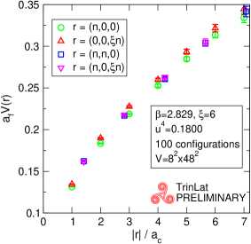
Figure 1: Static potential for $\xi=6$, with tree level $c_{\mu\nu}$ in the action.

Preliminary results show that 1-loop corrections are $O(10^{-2})$ after tadpole subtraction, confirming that analytic control is very important.

4 Including quarks

When including fermions, avoiding $O(a_{c})$ discretization errors is the main problem when dealing with asymmetric discretizations [6]. To circunvent this we choose a formulation which includes up to $4^{\rm th}$ derivative terms [7]. The fermion action reads

$$S_{q} = \bar{\psi}\left(m+\sum_{c}(\gamma_{c}\Delta^{(1,{\rm i})}_{c}+sa_{c}^{3}\Delta^{(4)}_{c})\right.$$

$$+ \left.\sum_{f}(\gamma_{f}\Delta^{(1)}_{f}+\frac{ra_{f}}{2}\Delta^{(2)}_{f})\right)\psi$$

where the regular Wilson discretization is used for the fine axis while up to $4^{\rm th}$ order corrections are included in the coarse directions [7].

5 Outlook & Developments

We have shown how 2+2 lattice QCD can be relevant to useful physics and feasible, although parameter tuning is necessary. Our formulation of lattice perturbation theory gives fine control over renormalization and a framework for the calculation of matrix elements. Moreover, the quark lagrangian can be tuned using the same techniques, allowing interesting prospectives for the method [5].

References

• [1] M.Alford, T.R.Klassen and P.Lepage, Nucl. Phys. B 496 (1997) 377; C.J.Morningstar and M.J.Peardon, Phys. Rev.D 56 (1997) 4043.
• [2] J. Shigemitsu et al., hep-lat/0207011; J. Shigemitsu et al., these proceedings, hep-lat/0208062.
• [3] M.Alford et al.,Phys.Rev.D63 (2001) 074501.
• [4] I. T. Drummond et al., hep-lat/0208010.
• [5] TrinLat Collaboration, in preparation.
• [6] S. Groote, J. Shigemitsu, Phys.Rev. D62 (2000) 014508; J. Harada et al., Phys.Rev. D64 (2001) 074501.
• [7] H. W. Hamber, C. M. Wu, Phys. Lett. B 127 (1983) 119; Phys. Lett. B 133 (1983) 351.