Towards a strong-coupling theory of QCD at finite density

Abstract

We apply strong-coupling perturbation theory to the QCD lattice Hamiltonian. We begin with naive, nearest-neighbor fermions and subsequently break the doubling symmetry with next-nearest-neighbor terms. The effective Hamiltonian is that of an antiferromagnet with an added kinetic term for baryonic “impurities,” reminiscent of the $t$–$J$ model of high-$T_{c}$ superconductivity. As a first step, we fix the locations of the baryons and make them static. Following analyses of the $t$–$J$ model, we apply large-$N$ methods to obtain a phase diagram in the $N_{c},N_{f}$ plane at zero temperature and baryon density. Next we study a simplified $U(3)$ toy model, in which we add baryons to the vacuum. We use a coherent state formalism to write a path integral which we analyze with mean field theory, obtaining a phase diagram in the $(n_{B},T)$ plane.

Color superconductivity [1] at high density is so far a prediction only of weak-coupling analysis, valid (if at all) only at very high densities. We seek confirmation from methods that do not depend on weak coupling, as well as an extension to the regime of moderate densities. Since Euclidean Monte Carlo methods are unavailable when the chemical potential is non-zero, we turn to the strong-coupling limit of QCD; harking back to the early days of lattice gauge theory, we work in the Hamiltonian formulation. We derive an effective Hamiltonian for color-singlet states that takes the form of an antiferromagnet with a kinetic term for baryons. This effective Hamiltonian is very difficult to study. As a first step, we fix the position of the baryons and study mesonic excitations in the baryonic background. Coherent-state methods then enable us to derive equivalent models that are tractable in various limits of large $N_{c}$ and/or $N_{f}$. We benefit from the considerable work done on antiferromagnets in the context of large-$T_{c}$ superconductors [2, 3, 4], as well as from the early work of the SLAC group [5] and of Smit [6] on strong-coupling QCD.

1 The effective Hamiltonian

The lattice gauge Hamiltonian is composed of electric, magnetic, and fermion terms,

$$H=H_{E}+H_{U}+H_{F},$$ (1)

where the first term is the unperturbed Hamiltonian in the strong coupling limit,

$$H_{E}=\frac{1}{2}g^{2}\sum_{{\bf n}\mu}E_{{\bf n}\mu}^{2}.$$ (2)

The ground state sector of $H_{E}$ is highly degenerate, consisting of of all states with zero electric flux, whatever their fermion content,

$$|0\rangle|\chi\rangle_{F}=\left[\prod_{{\bf n}\mu}|E_{{\bf n}\mu}^{2}=0\rangle\right]|\chi\rangle_{F}.$$ (3)

Neglecting the magnetic term, which only contributes in high order, we perturb with the fermion kinetic term,

$$H_{F} = -i\sum_{{\bf n}\mu}\psi^{{\dagger}}_{\bf n}\alpha_{\mu}$$ (4)

$$\quad\times\sum_{j>0}D(j)\left(\prod U_{{\bf n}+k\hat{\mu},\mu}\right)\psi_{{\bf n}+j\mu}$$

We use four-component fermions with a general (diagonal) kernel $D(j)$. This is the best we can do, since domain-wall fermions are unavailable to us at strong coupling [7] and there is no Hamiltonian overlap formalism [8]. We will discuss the properties of these fermions in a moment.

The degeneracy is lifted in second order via diagonalization of an effective Hamiltonian,

$$H_{{\rm eff}}^{(2)} = \sum_{{\bf n}\mu j}K(j)\left(s_{\eta}^{\mu}\right)^{j+1}\left(\psi^{{\dagger}}M^{\eta}\psi\right)_{\bf n}$$ (5)

$$\qquad\times\left(\psi^{{\dagger}}M^{\eta}\psi\right)_{{\bf n}+j\hat{\mu}},$$

where $s_{\eta}^{\mu}$ is a sign factor and $K(j)$ is a new kernel. The effective Hamiltonian contains fermion bilinears at each site,

$$Q^{\eta}_{\bf n}=\left(\psi^{{\dagger}}M^{\eta}\psi\right)_{\bf n},$$ (6)

where the $M^{\eta}$ matrices act on the Dirac and the flavor indices, $M^{\eta}=\Gamma^{A}\otimes\lambda^{a}$. The operators $Q^{\eta}_{\bf n}$ generate a $U(4N_{f})$ algebra. If we fix the baryon number $B$ on a site, the color-singlet states on that site make up an irreducible representation of this algebra, whose Young tableau has $m=B+2N_{f}$ rows and $N_{c}$ columns (see Fig. 1).

Figure 1: Young tableau for single-site states with $B=m-2N_{f}$.

Expressed in terms of $Q^{\eta}_{\bf n}$, the effective Hamiltonian is an antiferromagnet. If the kernel $D(j)$ is chosen to give nearest-neighbor couplings only, $H_{{\rm eff}}^{(2)}$ will take the form

$$H_{{\rm eff}}^{(2)}=K(1)\sum_{{\bf n}\mu}Q^{\eta}_{\bf n}Q^{\eta}_{{\bf n}+\hat{\mu}}.$$ (7)

This antiferromagnet has the accidental $U(4N_{f})$ symmetry of naive fermions, which is responsible for part of the doubling problem. The even-$j$ terms in (5) break this symmetry to $SU(N_{f})\times SU(N_{f})\times U(1)_{V}\times U(1)_{A}$, which [apart from the unbreakable axial $U(1)$] is the desired continuum symmetry. Since we are interested in strong coupling where the free fermion dispersion relation is of no interest, this might be a good-enough partial solution of the doubling problem.

The theory of $H_{{\rm eff}}^{(2)}$ contains only static baryons, which make their presence felt through fixing the rep of $U(4N_{f})$ on each site. These baryons can move in the next order in perturbation theory (only if $N_{c}=3$—a fortunate special case). The effective Hamiltonian in third order is

$$H_{{\rm eff}}^{(3)} = -i\sum_{j{\bf n}\mu}\tilde{K}(j)b_{\bf n}^{{\dagger}I}\left[\alpha_{\mu}\otimes\alpha_{\mu}\otimes\alpha_{\mu}\right]_{II^{\prime}}b_{{\bf n}+j\hat{\mu}}^{I^{\prime}}$$ (8)

$$\quad+h.c.,$$

where the baryon operators are the color singlets $b^{I}=\epsilon_{\alpha\beta\gamma}\psi_{\alpha}^{a}\psi_{\beta}^{b}\psi_{\gamma}^{c}$ that belong to the rep of $U(4N_{f})$. The simple form of $H_{{\rm eff}}$ is deceptive, for the $b^{I}$’s are composite and hence do not obey canonical anticommutation relations.

For nearest-neighbor fermions, the usual spin diagonalization [5] gives a simplified Hamiltonian,

$$H_{{\rm eff}}^{(3)}=-i\tilde{K}(1)\sum_{{\bf n}\mu}b_{\bf n}^{{\dagger}I}b_{{\bf n}+j\hat{\mu}}^{I}\eta_{\mu}({\bf n})+h.c.$$ (9)

The complete Hamiltonian $H_{{\rm eff}}^{(2)}+H_{{\rm eff}}^{(3)}$ resembles that of the $t$–$J$ model, which represents the strong-binding limit of the Hubbard model and is much studied in connection with high-$T_{c}$ superconductivity [9]. But our Hamiltonian is much more complex.

2 Static baryons

Let us beat a strategic retreat to the second-order theory, where baryons constitute a static background. If we begin with the nearest-neighbor model, in a state with no baryons, then the effective Hamiltonian (7) is that of a $U(4N_{f})$ antiferromagnet with spins in a rep specified by $N_{c}$ and by $m=2N_{f}$ (which can vary from site to site). This can be studied in the limits of large $N_{f},N_{c}$ by various transformations [2, 3, 4, 9], and the result—still for $B=0$—is the phase diagram in Fig. 2.

Figure 2: Phase diagram for the nn antiferromagnet at $T=0$

(Note that the coupling constant $K(1)$ is just a scale, which has no effect at $T=0$.) The large-$N_{f}$ phase is disordered, and will not concern us. The location of the phase boundary can be established by studying a Schwinger boson representation of the $U(4N_{f})$ spins, and its slope turns out to be $N_{c}/N_{f}=0.31$; this means that the QCD vacuum is safely in the ordered phase for any reasonable number of flavors.

The ordered phase is conveniently studied in a $\sigma$ model representation, which comes from rewriting (7) in a basis of spin coherent states [4]. (This is valid for any $N_{c},N_{f}$ but proves soluble in the $N_{c}\to\infty$ limit.) The degrees of freedom of the $\sigma$ model are the $N\times N$ matrices (with $N\equiv 4N_{f}$)

$$Q_{\bf n}=U_{\bf n}\Lambda U_{\bf n}^{{\dagger}},$$ (10)

where

$$\Lambda=\left(\begin{array}[]{cc}1_{N/2}&0\\ 0&-1_{N/2}\end{array}\right).$$ (11)

The field $U_{\bf n}$ runs over the group $U(N)$, and the manifold covered by $Q_{\bf n}$ is the coset space $U(N)/[U(N/2)\times U(N/2)]$. The action of the $\sigma$ model (in continuous time) is

$$S=\int_{0}^{\beta}d\tau\left[\frac{N_{c}}{2}\sum_{{\bf n}}{\rm Tr}\,\Lambda U^{{\dagger}}_{{\bf n}}\partial_{\tau}U_{{\bf n}}-H(Q(\tau))\right],$$

(12)

where, in terms of the matrices $Q_{\bf n}$, the nearest-neighbor Hamiltonian takes the form

$$H=\left(\frac{N_{c}}{2}\right)^{2}K(1)\sum{\rm Tr}\,Q_{\bf n}Q_{{\bf n}+\hat{\mu}}.$$ (13)

Clearly as $N_{c}\to\infty$ the ground state is the classical minimum of $H$, in which on all sites $Q_{\bf n}=Q_{0}$, which can be rotated to $Q_{\bf n}=\Lambda$. Thus the symmetry is spontaneously broken as $U(N)\to U(N/2)\times U(N/2)$, with $N^{2}/2$ Goldstone bosons [6].

We now restore next-nearest-neighbor couplings, viz.

$$H^{\prime}=\frac{K(2)}{2}\left(\frac{N_{c}}{2}\right)^{2}\sum_{{\bf n}\mu}Q^{\eta}_{{\bf n}}Q^{\eta}_{{\bf n}+2\hat{\mu}}s^{\mu}_{\eta},$$ (14)

where $Q^{\eta}_{{\bf n}}=2{\rm Tr}\,M^{\eta}Q_{\bf n}$. The symmetry of the theory, as discussed above, is $U(N_{f})\times U(N_{f})$; the classical minimum is at $Q_{\bf n}=\gamma_{0}$, which breaks all the axial generators and leaves the vector $U(N_{f})$ unbroken. This is what we would expect for the ground state in the vacuum sector.

3 Adding baryons

The $B=0$ states considered above were specified by choosing the $m=2N_{f}$ rep on each site. Choosing a different rep adds (or subtracts) baryons on a site-by-site basis. For instance, we can add a single baryon by adding a row to the Young tableau (Fig. 3).

Figure 3: Adding one baryon to a site in the $N_{f}=1$ theory [a $U(4)$ antiferromagnet]

One can similarly add baryons on an entire sublattice. The $N_{c}\to\infty$ limit directs us to find the classical ground state of the Hamiltonian, which always breaks the symmetry spontaneously along the lines shown in the section above. We can study the effects of the fluctuations by doing mean field theory for finite $N_{c}$. To do this, we drop the kinetic term in (12) and go to $T\not=0$ by calculating the resulting classical partition function.

4 Mean field theory

In MF theory, we write down a trial Hamiltonian and calculate a variational free energy $\Phi$. The simplest trial Hamiltonian, containing no site–site correlations, is

$$H_{0}=\sum_{\bf n}\vec{Q}_{\bf n}\cdot\vec{h}_{\bf n},$$ (15)

where the magnetic fields $\vec{h}_{\bf n}$ are variational parameters. (We write $\vec{Q}_{\bf n}$ for the vector whose $N^{2}$ components are $Q^{\eta}_{\bf n}$.) The free energy obeys $F\leq\Phi$ with

$$\Phi = -\sum_{\bf n}\log\left(\int dQ_{\bf n}\,e^{-K\vec{Q}_{\bf n}\cdot\vec{h}_{\bf n}}\right)$$ (16)

$$\quad+K\sum_{\langle{\bf m}{\bf n}\rangle}\vec{\mu}_{\bf m}\cdot\vec{\mu}_{\bf n}-\sum_{\bf n}\vec{\mu}_{\bf n}\cdot\vec{h}_{\bf n}$$

Here $K=\beta\frac{K(1)}{2}\left(\frac{N_{c}}{2}\right)^{2}$ and $\vec{\mu}$ is the magnetization,

$$\vec{\mu}_{\bf n}=\frac{\int dQ_{\bf n}\,e^{-\vec{Q}_{\bf n}\cdot\vec{h}_{\bf n}}\vec{Q}_{\bf n}}{\int dQ_{\bf n}\,e^{-\vec{Q}_{\bf n}\cdot\vec{h}_{\bf n}}}.$$ (17)

Note that the integration measure $dQ_{\bf n}$ depends on the $U(N)$ representation chosen for site ${\bf n}$.

We minimize $\Phi$ with respect to $\{\vec{h}_{\bf n}\}$ and get the mean field equations,

$$\vec{\mu}_{\bf n}=\frac{\int dQ_{\bf n}\,e^{-K\vec{Q}_{\bf n}\cdot\sum_{{\bf m}({\bf n})}\vec{\mu}_{\bf m}}\vec{Q}_{\bf n}}{\int dQ_{\bf n}\,e^{-K\vec{Q}_{{\bf n}}\cdot\sum_{{\bf m}({\bf n})}\vec{\mu}_{\bf m}}}.$$ (18)

If all sites are in the same rep of $U(N)$, then the bipartite nature of the antiferromagnetic system gives two coupled sets of MF equations. Otherwise one gets as many coupled MF equations as there are inequivalent sites.

After solving for $\vec{\mu}_{\bf n}$ we evaluate $\Phi$ via

$$\Phi = -\sum_{\bf n}\log\left(\int dQ\,e^{-K\vec{Q}_{\bf n}\cdot\sum_{{\bf m}({\bf n})}\vec{\mu}_{\bf m}}\right)$$ (19)

$$\quad-K\sum_{\langle{\bf m}{\bf n}\rangle}\vec{\mu}_{\bf n}\cdot\vec{\mu}_{\bf m}.$$

We seek the global minimum of $\Phi$. Once we find it, we can examine its symmetry properties and identify the phase favored at temperature $T$.

5 $U(3)$, a toy model

The $N_{f}=1$ theory, the $U(4)$ antiferromagnet (with impurities), contains many degrees of freedom in which to do mean field theory. A simpler non-trivial model is a toy model with $U(3)$ symmetry, which does not correspond to an actual value of $N_{f}$. The most symmetric $B=0$ state in this model cannot have $B=0$ on every site, but must alternate between the reps corresponding to $B=\pm 1/2$ (see Fig. 4).

Figure 4: The $B=0$ state in the $U(3)$ toy model

A $B\not=0$ state is specified by breaking the alternating pattern, as in Fig. 5.

Figure 5: Adding a baryon in the $U(3)$ toy model

We in fact create a non-zero density of baryons by adding a row to one or more sublattices, forming a lattice with a unit cell of $2\times 2\times 2$ sites. The unit cell may contain sites with $m=1$, 2, or even 3. For $m=1,2$ the manifold of $\vec{Q}_{\bf n}$ is $U(3)/[U(2)\times U(1)]$, while for $m=3$, the singlet state, we have $\vec{Q}_{\bf n}=0$.

The form of $U_{{\bf n}}$ for a site with $m=2$ is $U_{{\bf n}}=e^{A_{{\bf n}}}$, with

$$A=\left(\begin{array}[]{ccc}0&0&a_{1}\\ 0&0&a_{2}\\ -a^{*}_{1}&-a^{*}_{2}&0\end{array}\right).$$ (20)

We write

$$a_{1} = \rho\cos(\theta/2)e^{i\alpha_{1}}$$

$$a_{2} = \rho\sin(\theta/2)e^{i\alpha_{2}},$$ (21)

with $0<\rho,\theta<\pi$ and $0<\alpha_{1,2}<2\pi$. With these definitions, $\vec{Q}$ is given by

$$\vec{Q}=-2\left(\begin{array}[]{c}-\frac{1}{\sqrt{6}}\\ \sin^{2}\rho\sin\theta\cos\phi\\ -\sin^{2}\rho\sin\theta\sin\phi\\ \sin^{2}\rho\cos\theta\\ \sin 2\rho\cos\theta/2\cos\left(\frac{1}{2}(\psi+\phi)\right)\\ -\sin 2\rho\cos\theta/2\sin\left(\frac{1}{2}(\psi+\phi)\right)\\ \sin 2\rho\sin\theta/2\cos\left(\frac{1}{2}(\psi-\phi)\right)\\ -\sin 2\rho\sin\theta/2\sin\left(\frac{1}{2}(\psi-\phi)\right)\\ -\sqrt{3}\left(\cos^{2}\rho-\frac{1}{3}\right)\end{array}\right)$$ (22)

Here $\phi\equiv\alpha_{1}-\alpha_{2}$ and $\psi=\alpha_{1}+\alpha_{2}$, with $0<\psi<4\pi$ and $0<\phi<2\pi$. The induced measure on the four-dimensional manifold turns out to be

$$dQ=(1-\cos^{2}\rho)\cos\rho\,d(\cos\rho)d(\cos\theta)\frac{d\phi}{2\pi}\frac{d\psi}{4\pi}$$ (23)

An example: For the $B=0$ case shown in Fig. 4, the inequivalent sites are just the even and odd sublattices. The corresponding MF equations are

$$\vec{\mu}_{1} = \frac{\int dQ\,e^{-6K\vec{Q}\cdot\vec{\mu}_{2}}\vec{Q}}{\int dQ\,e^{-6K\vec{Q}\cdot\vec{\mu}_{2}}}$$ (24)

$$\vec{\mu}_{2} = -\frac{\int dQ\,e^{+6K\vec{Q}\cdot\vec{\mu}_{1}}\vec{Q}}{\int dQ\,e^{+6K\vec{Q}\cdot\vec{\mu}_{1}}}.$$

Cases with $B\not=0$ will give more coupled sets of MF equations, according to the number of inequivalent sites in the unit cell.

For each baryonic configuration we obtain a phase transition as a function of temperature. In some cases it is first order and in others, second order. In all cases the symmetry breakdown at low temperature is $U(3)\to U(3)/[U(2)\times U(1)]$. As we increase the baryon density the transition temperature decreases, but it never vanishes; MF theory always breaks symmetry at $T=0$, even in one dimension. We summarize our findings in the phase diagram in the temperature–density plane shown in Fig. 6.

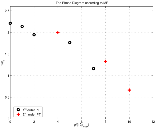
Figure 6: Classical phase transition of the $U(3)$ antiferromagnet with a density of baryon impurities. The ordinate is proportional to temperature, while the abscissa is baryon density in units of the maximum saturation density $\rho_{\rm max}$.

The future holds, we hope, the removal of the various approximations that led from QCD to the $U(3)$ toy model. To begin with, we must do better than classical mean field theory and include the quantum kinetic term in the $\sigma$ model (12). The $U(3)$ model must be generalized to the $U(4N_{f})$ symmetry group of naive fermions, which should be broken to $U(N_{f})\times U(N_{f})$ by the nnn coupling. Going beyond the static baryon picture, we can disorder the baryon background by a replica method; eventually dynamical baryons should be included with the third-order kinetic term. Once the theory becomes realistic enough, we can compare the results at each step to the weak-coupling predictions of color superconductivity with various values of $N_{f}$ [10].

There is, however, a limitation inherent in the strong-coupling theory. As we saw in the mean-field analysis above, one is easily misled into filing the lattice with baryons to saturation. The baryon density is limited according to

$$\frac{B}{V}<\frac{2N_{f}}{a^{3}},$$ (25)

and strong coupling means large lattice spacing $a$. It is possible that color superconductivity will not show up at any density short of saturation. In that case we will have to content ourselves with a new effective theory for baryonic matter, short of the transition to quark matter.

References

- [1] K. Rajagopal and F. Wilczek, arXiv:hep-ph/0011333.
- [2] I. Affleck, Nucl. Phys. B 257 (1985) 397; J. B. Marston and I. Affleck, Phys. Rev. B 39 (1989) 11538.
- [3] D. P. Arovas and A. Auerbach, Phys. Rev. B 38 (1988) 316 .
- [4] N. Read and S. Sachdev, Nucl. Phys. B 316 (1989) 609; Phys. Rev. B 42 (1990) 4568.
- [5] B. Svetitsky, S. D. Drell, H. R. Quinn and M. Weinstein, Phys. Rev. D 22 (1980) 490.
- [6] J. Smit, Nucl. Phys. B 175 (1980) 307.
- [7] R. C. Brower and B. Svetitsky, Phys. Rev. D 61 (2000) 114511 [arXiv:hep-lat/9912019].
- [8] M. Creutz, I. Horvath and H. Neuberger, Nucl. Phys. Proc. Suppl. 106 (2002) 760 [arXiv:hep-lat/0110009].
- [9] A. Auerbach, Interacting electrons and quantum magnetism (Springer-Verlag, 1994).
- [10] T. Schäfer, Nucl. Phys. B 575 (2000) 269 [arXiv:hep-ph/9909574].