New Algorithm of the Finite Lattice Method for the High-temperature Expansion
of the Ising Model in Three Dimensions

Abstract

We propose a new algorithm of the finite lattice method to generate the high-temperature series for the Ising model in three dimensions. It enables us to extend the series for the free energy of the simple cubic lattice from the previous series of 26th order to 46th order in the inverse temperature. The obtained series give the estimate of the critical exponent for the specific heat in high precision.

The finite lattice methodEnting1977 ; Creutz1991 ; Arisue1984 is a powerful tool to generate the high- and low- temperature series for the spin models in the infinite volume limit. It avoids the tedious work of counting all the diagrams in the graphical method and reduce the problem to the calculation of the partition function. In two dimensions the total amount of the calculations for the finite lattice method increases exponentially with the maximum order $N$ of the series. On the other hand in three dimensions the total amount of the calculations grows exponentially with $N^{2}$ and except for some casesBhanot1994 ; Guttmann1994 ; Bhanot1992 ; Guttmann1993 ; Arisue1994 ; Arisue1995 ; Arisue1993 ; Bhanot1993 ; Guttmann1994b many of the expansion series have been calculated by the graphical method. Here we present a new algorithm of the finite lattice method for the high-temperature expansion in three dimensions in which the total amount of the calculation increase approximately exponentially with $N\log{N}$ and that enables us to generate the series to much higher orders than not only the standard algorithm of the finite lattice method but also the graphical method.

In the finite lattice method to generate the high-temperature series for the free energy in three dimensions we calculate the partition function $Z(l_{x}\times l_{y}\times l_{z})$ for the finite size lattices with $2(l_{x}+l_{y}+l_{z})\leq N$ and define recursivelyArisue1984

$$\phi(l_{x}\times l_{y}\times l_{z}) = \log{[Z(l_{x}\times l_{y}\times l_{z})]}$$ (1)

$$\!\!\!\!\!\!\!\!\!\!\!\!\!\!\!\!\!\!\!\!\!\!-\sum_{\stackrel{{\scriptstyle\scriptstyle l_{x}^{\prime}\leq l_{x},l_{y}^{\prime}\leq l_{y},l_{z}^{\prime}\leq l_{z},}}{{\scriptstyle l_{x}^{\prime}+l_{y}^{\prime}+l_{z}^{\prime}\neq l_{x}+l_{y}+l_{z}}}}\phi(l_{x}^{\prime}\times l_{y}^{\prime}\times l_{z}^{\prime})\;.$$

Here we use the notation for the lattice size such that the $1\times 1\times 1$ lattice means the unit cube composed of $2\times 2\times 2$ sites. The Boltzmann factor for each bond connecting the nearest neighbor sites $k$ and $k^{\prime}$ is expressed as

$$\exp\left(\beta s_{k}s_{k^{\prime}}\right)=\cosh\left(\beta\right)\left(1+ts_{k}s_{k^{\prime}}\right),$$ (2)

with $t=\tanh\left(\beta\right)$. We define the bond configuration as the set of bonds to which the factor $ts_{k}s_{k^{\prime}}$ in (2) is assigned while the factor $1$ is assigned to the other bonds of the finite size lattice. Non-vanishing contribution to the partition function comes only from the bond configuration in which the bonds form one or more closed loops. Each of the closed loops is a polymer in the standard cluster expansionMuenster1981 . Then the Taylor expansion of $\phi(l_{x}\times l_{y}\times l_{z})$ with respect to $t$ includes the contribution from all the clusters of polymers in the standard cluster expansion that can be embedded into the lattice of $l_{x}\times l_{y}\times l_{z}$ but cannot be embedded into any of its rectangular sub-lattices $l_{x}^{\prime}\times l_{y}^{\prime}\times l_{z}^{\prime}$Arisue1984 . The expansion series of the free energy density in the infinite volume limit is given by

$$f=\sum_{2(l_{x}+l_{y}+l_{z})\leq N}\phi(l_{x}\times l_{y}\times l_{z})$$ (3)

The expansion series of $\phi(l_{x}\times l_{y}\times l_{z})$ starts from the term of $t^{n}$ with $n=2(l_{x}+l_{y}+l_{z})$, which comes from the cluster of a single polymer (one closed loop of bonds) that have two intersections with any plane perpendicular to the lattice bonds. Thus it is enough to restrict the lattice sizes for the summation in (3) to those that satisfy $2(l_{x}+l_{y}+l_{z})\leq N$ to obtain the series for $f$ to order $t^{N}$.

In the standard algorithm of the finite lattice method the full partition function for the finite size lattice is calculated with all the bond configurations taken into account. The point of the new algorithm is that, in order to obtain the series to a given order, however, it is enough to consider only a restricted number of bond configurations. Let us consider the anisotropic model of the simple cubic Ising model with $\beta_{i}=J_{i}/k_{B}T$ and $t_{i}=\tanh{(\beta_{i})}$ ($i=x,y,z$). To obtain the series for $\phi(l_{x}\times l_{y}\times l_{z})$ to order $N_{z}=2l_{z}+\Delta N_{z}$ in $t_{z}$ we introduce in the new algorithm $\phi(l_{x}\times l_{y}\times l_{z},\Delta N_{z})$ defined recursively by

$$\phi(l_{x}\times l_{y}\times l_{z},\Delta N_{z}) = \log{[Z(l_{x}\times l_{y}\times l_{z},\Delta N_{z})]}$$ (4)

$$\!\!\!\!\!\!\!\!\!\!\!\!\!\!\!\!\!\!\!\!\!\!\!\!\!\!\!\!\!\!\!\!\!\!\!\!\!\!\!\!\!\!\!\!-\sum_{\stackrel{{\scriptstyle\scriptstyle l_{x}^{\prime}\leq l_{x},l_{y}^{\prime}\leq l_{y},l_{z}^{\prime}\leq l_{z},}}{{\scriptstyle l_{x}^{\prime}+l_{y}^{\prime}+l_{z}^{\prime}\neq l_{x}+l_{y}+l_{z}}}}\phi(l_{x}^{\prime}\times l_{y}^{\prime}\times l_{z}^{\prime},\Delta N_{z})\;.$$

Here the partition function $Z(l_{x}\times l_{y}\times l_{z},\Delta N_{z})$ is calculated only with the bond configurations taken into account that have orders $n_{z}{{}_{i}}$ in $t_{z}$ for the $i$-th layer perpendicular to the z-axis ($i=1,2,\cdots,l_{z}$) satisfying

$$\sum_{i=1}^{l_{z}}\max(n_{z}{{}_{i}},2)\leq 2l_{z}+\Delta N_{z}\;.$$ (5)

Examples of the bond configuration for $Z(l_{x}\times l_{y}\times l_{z},\Delta N_{z})$ that should be taken into account or should be neglected can be seen in Fig. 1.

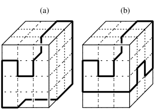
Figure 1: Examples of the bond configuration for $Z(l_{x}\times l_{y}\times l_{z},\Delta N_{z})$ with $l_{x}=3,l_{y}=3,l_{z}=4,\Delta N_{z}=2$. Example (a) has $n_{z}{{}_{1}}=2$, $n_{z}{{}_{4}}=2$, $n_{z}{{}_{3}}=4$, and $n_{z}{{}_{4}}=2$ and it should be taken into account, while (b) has $n_{z}{{}_{1}}=0$, $n_{z}{{}_{4}}=4$, $n_{z}{{}_{3}}=4$, and $n_{z}{{}_{4}}=2$ and it should be neglected.

It is easy to prove that any bond configuration for the partition function that has $\sum_{i=1}^{l_{z}}n_{z}{{}_{i}}\leq 2l_{z}+\Delta N_{z}$ but $\sum_{i=1}^{l_{z}}\max(n_{z}{{}_{i}},2)>2l_{z}+\Delta N_{z}$ does not contribute to the left hand side of (4) in the order lower than or equal to $N_{z}=2l_{z}+\Delta N_{z}$. For such a bond configuration at least one of the $n_{z}{{}_{i}}$’s should be zero, so they are disconnected configuration(composed of more than one polymer) or they can be embedded into a rectangular sub-lattice of the $l_{x}\times l_{y}\times l_{z}$ lattice and in either case they do not contribute to $\phi(l_{x}\times l_{y}\times l_{z},\Delta N_{z})$ in the order lower than or equal to $N_{z}=2l_{z}+\Delta N_{z}$. They can contribute to $\phi(l_{x}\times l_{y}\times l_{z},\Delta N_{z})$ in higher order than $N_{z}=2l_{z}+\Delta N_{z}$ by constituting the connected cluster of polymers together with other configurations with $n^{\prime}{{}_{z}{{}_{i}}}\geq 2$ for the layer $i$ with $n_{z}{{}_{i}}=0\;$. Then total order of the cluster of polymers has the order higher than $N_{z}=2l_{z}+\Delta N_{z}$.

The contribution of the bond configuration with $\{n_{z}{{}_{i}}\}$ to the partition function of the finite size lattice can be calculated by the transfer matrix formalism as

$$Z(\{n_{z}{{}_{i}}\})=V_{0,j_{1}}t_{z}^{n_{z}{{}_{1}}}V_{j_{1},j_{2}}t_{z}^{n_{z}{{}_{2}}}\cdots t_{z}^{n_{z}{{}_{l_{z}}}}V_{j_{l_{z}},0}\,.$$ (6)

Here $V_{j_{i},j_{i+1}}$ is the transfer matrix element with incoming $n_{z}{{}_{i}}$ spins and outgoing $n_{z}{{}_{\;i+1}}$ spins and the summations over the spin locations $j_{1},j_{2},\cdots$ of the $n_{z}{{}_{1}},n_{z}{{}_{2}},\cdots$ spins, respectively, are assumed in the right hand side of (6). This transfer matrix element itself is the partition function in two dimensions with $n_{z}{{}_{i}}+n_{z}{{}_{\;i+1}}$ spins attached, which can be calculated to any order in $t_{x}$ and $t_{y}$ efficiently by the site-by-site constructionEnting1980 ; Bhanot1990 . The amount of the calculation for each transfer matrix element is proportional to the combinatorial factor $C(\ (l_{x}+1)(l_{y}+1)\ ,n_{z}{{}_{i}}+n_{z}{{}_{\;i+1}})$, $2^{l_{x}}$ and $l_{x}l_{y}$, which are the number of the cases for attaching the $n_{z}{{}_{i}}+n_{z}{{}_{\;i+1}}$ spins to the $(l_{x}+1)(l_{y}+1)$ sites, the number of states in site-by-site construction for the partition function of the Ising model in two dimensions and the number of the relevant bonds, respectively.

To obtain the series to order $N$ in the isotropic model, we calculate the expansion series for each of the $\phi(l_{x}\times l_{y}\times l_{z})$’s defined by (1) in the anisotropic model to order $t_{x}^{N_{x}}t_{y}^{N_{y}}t_{z}^{N_{z}}$ with $N_{x}+N_{y}+N_{z}=N$ using the new algorithm described above and set $t_{x}=t_{y}=t_{z}=t$ finally. When we use the new algorithm for each lattice size $l_{x}\times l_{y}\times l_{z}$ and each of the orders $N_{x},N_{y},N_{z}$, we can make the simultaneous exchange of the lattice axes and corresponding orders as $(l_{x}\times l_{y}\times l_{z};N_{x},N_{y},N_{z})\to(l_{x}\times l_{z}\times l_{y};N_{x},N_{z},N_{y})$ or $(l_{x}\times l_{y}\times l_{z};N_{x},N_{y},N_{z})\to(l_{y}\times l_{z}\times l_{x};N_{y},N_{z},N_{x})$ that have the chance to reduce the amount of the calculation for the transfer matrix elements.

Figure 2: Total amount of the calculation to generate the series to order $N$ by the old algorithm and the new algorithm of the finite lattice method.

We estimate the total amount of the calculation time $T_{\mathrm{calc}}(N)$ to generate the free energy series to order $N$ by listing up all the transfer matrices needed and summing up the estimated time to calculate each of the matrices, which is plotted in Fig. 2 together with the estimated total calculation time for the old algorithm of the finite lattice method. The numerical estimation for the new algorithm agrees well with the actually used calculation time for $N\leq 46$. We see that the calculation time for the old algorithm grows exponentially with $N^{2}$, while that for the new algorithm can be fitted by $A\exp{(BN\log{N}+CN+D\log{N})}$ with $B\sim 0.15$, $C\sim-0.24$ and $D\sim 3.6$. We can simply understand this $\exp(BN\log N+...)$ behavior as follows. The maximum size of the lattice to be taken into account is $l_{x}=l_{y}=l_{z}=N/6$, for which $\Delta N_{z}=0$ and we have only to consider the bond configurations with $n_{z}{{}_{i}}=2$ for all $i=1,2,\cdots,l_{z}$. The largest amount of the calculation is to be paid for the partition function of the lattice that has smaller size of $l_{x}\sim l_{y}\sim l_{z}\sim N/12$ for which the maximum of $n_{z}{{}_{i}}+n_{z}{{}_{\;i+1}}$ is about $N/6$ and the product of the above factors is approximately proportional to $\exp\left(BN\log{N}+CN+D\log{N}\right)$ with $B=1/6$ for large $N$.

Table 1: High-temperature expansion coefficients for the free energy density of the simple cubic Ising model.

$n$	$\qquad a_{n}$
$2$	$\qquad 0$
$4$	$\qquad 3$
$6$	$\qquad 22$
$8$	$\qquad 375/2$
$10$	$\qquad 1980$
$12$	$\qquad 24044$
$14$	$\qquad 319170$
$16$	$\qquad 18059031/4$
$18$	$\qquad 201010408/3$
$20$	$\qquad 5162283633/5$
$22$	$\qquad 16397040750$
$24$	$\qquad 266958797382$
$26$	$\qquad 4437596650548$
$28$	$\qquad 525549581866326/7$
$30$	$\qquad 6448284363491202/5$
$32$	$\qquad 179577198475709847/8$
$34$	$\qquad 395251648062268272$
$36$	$\qquad 21093662188820520521/3$
$38$	$\qquad 126225408651399082182$
$40$	$\qquad 4569217533196761997785/2$
$42$	$\qquad 291591287110968623857940/7$
$44$	$\qquad 8410722262379235048686604/11$
$46$	$\qquad 14120314204713719766888210$

Using the new algorithm of the finite lattice method we have calculated the high-temperature series for the free energy density of the simple cubic Ising model to order $N=46$. The coefficients of the obtained series

$$f=3\cosh{(\beta)}+\sum_{n}a_{n}t^{n};\quad t=\tanh{(\beta)}$$ (7)

are listed in Table 1. They agree with those given by Bhanot et alBhanot1994 to order $N=24$ and by Guttmann and EntingGuttmann1994 to order $N=26$. We have add ten new terms to these previous series. To obtain the series of order $N=26$ in our new algorithm we needed only the computer memory of 1 MBytes and the CPU-time of 5 minutes in a standard PC and to order $N=46$ we used the total memory of 2 GBytes and the CPU time of 25 hours in CP-PACS at Tsukuba University.

Following is the result of the preliminary analysis of the series for the specific heat $C(t)=\sum_{n}c_{n}t^{n}$. We plot in Fig. 3 the critical exponent $\alpha$ versus the critical value $\beta_{c}$ for the first order inhomogeneous differential approximants of the series of $N=40$–$46$. From the linear dependence of $\alpha$ on $\beta_{c}$ we find $\alpha=0.1045(1)$ or $\alpha=0.1077(2)$ at the value $\beta_{c}=0.22165459(10)$Blote1999 or $\beta_{c}=0.2216595(15)$Ito2000 obtained in the recent Monte Carlo simulations. The second order inhomogeneous differential approximants give almost the same value.

Figure 3: Critical exponent $\alpha$ versus the critical value $\beta_{c}$ for the inhomogeneous differential approximants of the first order.

Figure 4: Sequence $\alpha_{n}$ plotted versus $1/n$.

We also made the ratio analysis. The sequence $\alpha_{n}=(t_{c}^{2}c_{2n}/c_{2n-2}-1)n+1$, which is expected to behave as $\alpha+b/n^{\Delta}+c/n+\cdots$ with the correction-to-scaling exponent $\Delta\sim 0.5$, is plotted versus $1/n$ in Fig. 4 for $\beta_{c}=0.22165459$. The sequence for $n=14$–$23$ given by the new 10 coefficients has a bit different slope from the sequence for $n\leq 13$ given by the previously obtained series. Three-parameter fitting of the newly obtained sequence for $\beta_{c}=0.22165459$ gives $\alpha=0.1036(10)$, $b=-0.007(10)$ and $c=0.17(2)$ for $\Delta=0.5$. As for the case of $\beta_{c}=0.2216595$ it gives $\alpha=0.1082(14)$, $b=-0.033(10)$ and $c=0.21(2)$. These estimated values of $\alpha$ by the inhomogeneous differential approximation and by the ratio method are not inconsistent with each other. We see, on the other hand, that the estimated values of $\alpha$ depends crucially on the value of $\beta_{c}$ and in order to determine $\alpha$ precisely in these biased method we need more precise value of $\beta_{c}$. We also notice that the correction-to-scaling term is very small, which was already pointed out in the analysis of the shorter seriesBhanot1994 ; Guttmann1994 .

From the hyperscaling relation $\alpha=2-d\nu$ the high-temperature series for the second moment correlation length gives $\alpha=0.1088(39)$Butera2002 and $\alpha=0.1096(5)$Campostrini2002 and the $\epsilon$-expansion gives $\alpha=0.1088(39)$Guida1997 . More direct estimation of $\alpha=0.110(2)$ was also given by the high-temperature series for the magnetic susceptibility of the antiferromagnetic critical pointCampostrini2002 . We note that our estimated value of $\alpha$ using $\beta_{c}=0.22165459$ is not consistent with these values but the value using $\beta_{c}=0.2216595$ is rather closer to these values.

The basic idea presented here in the new algorithm of the finite lattice method can be applied to the high-temperature expansion of other quantities such as the magnetic susceptibility and the correlation length for the Ising model in three dimensions and it can also be applied to the models with continuous spin variables such as the XY model in three dimensions. Furthermore the idea can be used in the low-temperature expansion for the spin models in three dimensions. We can expect that it will enable us to generate the expansion series in much higher orders compared with the presently available series.

References

- (1) T. de Neef and I. G. Enting, J. Phys. A 10, 801 (1977); I. G. Enting, J. Phys. A 11, 563 (1978); Nucl. Phys. B (Proc. Suppl.) 47, 180 (1996).
- (2) H. Arisue and T. Fujiwara, Prog. Theor. Phys. 72, 1176 (1984); H. Arisue, Nucl. Phys. B (Proc. Suppl.) 34, 240 (1994).
- (3) M. Creutz, Phys. Rev. B 43, 10659 (1991).
- (4) G. Bhanot, M. Creutz, U. Glässner and K. Schilling, Phys. Rev. B 49, 12909 (1994).
- (5) A. J. Guttmann and I. G. Enting, J. Phys. A 27 8007 (1994).
- (6) G. Bhanot, M. Creutz, J. Lacki, Phys. Rev. Lett. 69, 1841 (1992).
- (7) A. J. Guttmann and I. G. Enting, J. Phys. A 26 807 (1993).
- (8) H. Arisue and T. Fujiwara, Nucl. Phys. B 285[FS19] 253 (1987) H. Arisue, Phys. Letters B 322 224 (1994)
- (9) H. Arisue and K. Tabata, Nucl. Phys. B 435 555 (1995)
- (10) H. Arisue, Phys. Letters B 313 187 (1993)
- (11) G. Bhanot, M. Creutz, U. Glässner, I. Horvath, J. Lacki, K. Schilling and J. Weckel, Phys. Rev. B 48, 6183 (1993).
- (12) A. J. Guttmann and I. G. Enting, J. Phys. A 27 5801 (1994).
- (13) G. Münster, Nucl. Phys. B180[FS2] 23 (1981).
- (14) I. G. Enting, J. Phys. A 13 3713 (1980).
- (15) G. Bhanot, J. Stat. Phys. 60, 55 (1990).
- (16) H. W. J. Blöte, L. N. Shchur and A. L. Talapov, Int. Journ. Mod. Phys. C 10, 137 (1999).
- (17) N. Ito, K. Hukushima, K. Ogawa and Y. Ozeki, J. Phys. Soc. Japan, 69, 1931 (2000).
- (18) P. Butera and M. Comi, Phys. Rev. B 65, 144431 (2002).
- (19) M. Campostrini, P. Rossi and E. Vicari, A. Pelissetto, Phys. Rev. E 65 066127 (2002).
- (20) R. Guida and J. Zinn-Justin, Nucl. Phys. B 489, 626 (1997); J. Phys. A 31, 8103 (1998).