Screening of hot gluon
$\sim$ Lattice study of gluon screening masses $\sim$

A. Nakamura, I. Pushkina^a, T. Saito and S. Sakai^b

Abstract

We calculate electric and magnetic masses of gluons between $T=T_{c}$ and $6T_{c}$ using lattice QCD (quantum chromodynamics) in the quench approximation for color $SU(3)$. We find that magnetic mass has finite values in this region, and the temperature dependence of the electric mass is consistent with that determined using the hard-thermal-loop perturbation. The hard-thermal-loop resummation improves significantly the magnitude of the electric mass comparing to the leading order perturbation. Both screening masses have little gauge parameter dependence.

We are expecting relativistic heavy-ion collisions to soon yield evidence of a quark-gluon plasma (QGP), by creating sufficiently high temperature to bring the system into the deconfining phase. This new form of matter is a prediction of QCD and will be studied for the first time in the laboratory. One of the most urgent theoretical tasks is to investigate the characteristics of gluons, the component of QGP that controls the force, at a finite temperature based on QCD. If we can calculate these features in a reliable manner, phenomenological observations, such as the jet quenching, may be analysed based on these knowledges.

There has been essential progress in the perturbative method of treating hot QCD. Using the hard-thermal-loop resummation technique[1], we can now handle plasma effects of gauge theories. The correct magnitude of the free energy from lattice QCD was reproduced by such a calculation[2, 3].

Fundamental quantities of the hot gluon plasma have been studied perturbatively. Electric mass is given by the lowest perturbative calculation as

$$m_{e,0}=\sqrt{\frac{N_{c}}{3}}gT.$$ (1)

Magnetic mass, $m_{m}$, is, however, beyond the scope of the perturbative treatment[4, 5]. It vanishes in the lowest perturbation, but if indeed $m_{m}=0$, the gluons are essentially unscreened, even if the electric mass is finite[6]. Also, zero magnetic mass causes serious infrared divergence and makes consistent theoretical treatment very difficult (see Chap.10.2 of Ref.[7]).

The maximum temperature accessible at RHIC or LHC is of the order of $1\mbox{GeV}$ or $5T_{c}$ which is far below the regions where the perturbative calculation can be safely applied. Therefore nonperturbative analysis is highly desirable in order to gain a quantitative understanding of the properties of QGP. Since the pioneering work for temperature dependencies of screening masses by Heller, Karsch and Rank for SU(2) color QCD[8], there have been several activities, but no $SU(3)$ lattice simulations of finite temperature gluon propagators in the literature. Indeed, calculations of gauge-dependent observables are very time-consuming and often unstable.

In this letter, we report the electric and magnetic screening masses of gluons at finite temperature measured in lattice simulations based on the SU(3) gauge theory, i.e., QCD in the quench approximation. We calculate gluon propagators; which allows direct comparison with perturbative calculations.

We calculate gluon correlation functions with finite momentum,

$$G_{\mu\nu}(P_{t},P_{x},P_{y},z)=\langle\mbox{Tr}A_{\mu}(P_{x},P_{y},P_{t},z)A_{\nu}(-P_{x},-P_{y},-P_{t},0)\rangle,$$ (2)

where gauge potentials $A_{\mu}$’s are evaluated from the link variables $U_{\mu}(x)\in$ SU(3) as $A_{\mu}(x)=(U_{\mu}(x)-U_{\mu}^{{\dagger}}(x))/2gi$. The calculation of propagators with finite momenta enables us to construct transverse and longitudinal components without ambiguity[9]; we define electric and magnetic parts of the gluon propagators as

$$\begin{array}[]{lll}G_{e}(P,z)&=&\frac{Z}{2}\left[G_{tt}(\frac{2\pi}{N_{x}},0,0,z)+G_{tt}(0,\frac{2\pi}{N_{y}},0,z)\right],\\ G_{m}(P,z)&=&\frac{Z}{2}\left[G_{xx}(0,\frac{2\pi}{N_{y}},0,z)+G_{yy}(\frac{2\pi}{N_{x}},0,0,z)\right],\end{array}$$ (3)

which correspond to standard projected propagators in perturbative calculations. Here $P_{\mu}$’s are lattice momenta, and the size of the lattice is given by $N_{x}N_{y}N_{z}N_{t}$. At a sufficiently large distance, they are expected to behave as

$$G_{e(m)}(z)\propto e^{-E_{e(m)}z}.$$ (4)

In order to quantize the theory and to extract gauge-dependent observables, we employ stochastic quantization $\grave{\mbox{a}}$ la Zwanziger[10],

$$\frac{dA_{\mu}^{a}}{d\tau}=-\frac{\delta S}{\delta A_{\mu}^{a}}+\frac{1}{\alpha}D_{\mu}(A)^{ab}\partial_{\nu}A_{\nu}^{b}+\eta_{\mu}^{a},$$ (5)

where $\tau$ is the Langevin time, the second term of the r.h.s. is the gauge fixing term, and $\eta$ represents Gaussian random noise. The gauge parameter is given by $\alpha$, and $\alpha=0$ corresponds to the Lorentz gauge. The lattice version of the algorithm was proposed in Ref.[11] as

$$U_{\mu}(x,\tau+\Delta\tau)=\omega^{\dagger}(x,\tau)e^{if_{\mu}^{a}t^{a}}U_{\mu}(x,\tau)\omega(x+\hat{\mu},\tau),$$ (6)

Here, $\omega$ means a gauge rotation matrix and $f$ a driving force.

$$f_{\mu}^{a}=-\frac{\partial S}{\partial A_{\mu}^{a}}\Delta\tau+\eta^{a}\sqrt{\Delta\tau},\hskip 28.45274pt\omega=e^{i\beta\Delta^{a}\tau^{a}\Delta\tau/\alpha}.$$ (7)

The gauge rotation step and Langevin step are executed alternately.

There are two reasons for using the stochastic gauge fixing method here: one is practical and the other is conceptual. Contrary to the standard Wilson-Mandula gauge fixing method[12], where an iterative procedure is applied and the number of iterations is unpredictable for large lattices, in algorithm (6), we repeat the steps of update and gauge rotation one after the other. There is no convergence problem of gauge fixing. Therefore we can precisely estimate CPU time. Moreover, this algorithm, which may change the gauge parameter $\alpha$, has an advantage in testing gauge independence. A conceptual problem is the Gribov ambiguity appearing in non-Abelian gauge theories[13]. Although our algorithm may not eliminate copies completely, Zwanziger’s stochastic gauge fixing algorithm maintains the gauge system inside the Gribov region[10, 14] if we start from the trivial configuration $\{A_{\mu}=0\}$.

We perform simulations on an $N_{x}N_{y}N_{z}N_{t}=20\times 20\times 32\times 6$ lattice with the standard Wilson gauge action. The physical temperature is tuned by changing the lattice cut-off scale 1/$a$[GeV], i.e., gauge coupling. The relation between gauge coupling and the lattice scale is estimated using the data in Ref.[15], which covers the range from $\beta=6/g^{2}=6$ to $7.1$. The confinement/deconfinement transition temperature is set to be 256 MeV[16]. Then we study the regions of $T/T_{c}=1\sim 6$. The Runge-Kutta algorithm is applied to reduce the finite Langevin step $\Delta\tau$ dependence[17]. We perform the simulation for a set of parameters with $\Delta\tau=0.03\sim 0.05$ and extrapolate all results linearly to $\Delta\tau=0$. The gauge parameter $\alpha$ is fixed to be one, except in the gauge dependence test.

We observe a large fluctuation of gauge propagators, particularly at large distances. We show in Fig.1 a typical behavior of gluon propagators $G(z)$ as a function of the Langevin step. In order to estimate the necessary number of Langevin update steps, we wait until $<G_{xx}(z)>$ and $<G_{yy}(z)>$ calculated in Eq.3 becomes equal to each other. A typical number of simulations is $0.2\sim 0.4$ million steps.

The dynamics of a gluon propagator is completely different in confinement and deconfinement regions[18]. In Fig.2, the gluon behavior is massive and we see that as distance $z$ increases, the mass of the propagator in confinement regions seems to become infinite; the gluon is completely screened in the confinement phase. Consequently, we cannot employ the assumption, Eq.(4). On the contrary, the propagator decreases exponentially at a long distance with a finite damping rate in the deconfinement region.

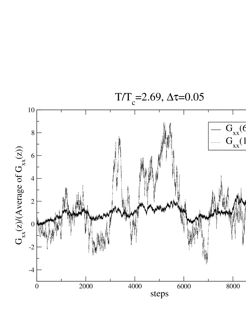
Figure 1: Typical gluon behavior with Langevin steps. We find that fluctuations of $G_{xx}(12)$ are much larger than those of $G_{xx}(6)$. In order to investigate the screening effect, long-range contribution should be adopted. Consequently we need a large number of statistics.

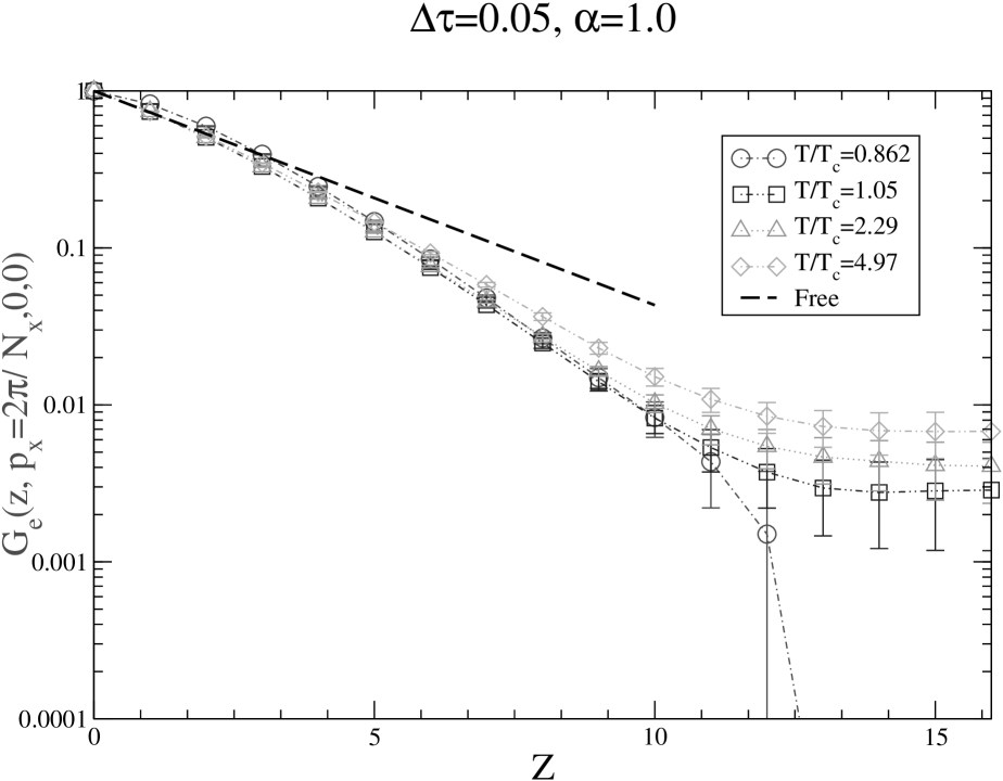
Figure 2: The electric propagator behavior in confinement (circle) and deconfinement phase (the others) with $P_{x}=\frac{2\pi}{N_{x}}$. We find all propagators become massive comparing with the free propagator (long dashed line). In confinement regions, the propagator at long distance seems to have infinite mass and vanishes, whereas we find that the propagator beyond $T_{c}$, has finite mass.

Figure 3: $\Delta\tau$ dependence of masses is slight. Therefore, obtaining a final value at $\Delta\tau=0$, we use the linear function for extrapolation. Here, it is important to apply the Runge-Kutta algorithm in order to suppress $\Delta\tau$ error.

To extract screening masses from the propagators we use the following fitting functions under the lattice periodic condition:

$$G_{e(m)}\sim\cosh(E_{e(m)}(p)(z-N_{z}/2)).$$ (8)

We employ values for $z>1/T(=N_{t}a)$, because a screening effect occurs in a sufficiently long range. Then, we obtain static mass from $E(p)$.

To get the final result at $\Delta\tau=0$, we must extrapolate with respect to Langevin step width. Fig.3 represents $E(p)$ measured here versus $\Delta\tau$. The slight dependences of $\Delta\tau$ cause us to use a linear function when fitting data.

Screening masses are physical and expected to be gauge independent. However, since the definition of the gluon propagator, Eq.(2) itself, is generally gauge dependent, it is nontrivial whether the screening masses are gauge invariant or not. In addition, since we fail to define the magnetic mass by a perturbative analysis, it is particularly important to check its gauge invariance. In Fig.4, we show the gauge parameter $\alpha$ dependence of electric and magnetic masses. The result strongly suggests that they are gauge independent and physical observables.

Figure 4: Gauge dependence graph for electric and magnetic screening masses. Gauge dependences of both screening masses are very slight in nonperturbative regions.

Figure 5: Temperature dependences of electric and magnetic screening masses. Dotted line was fitted based on the scaling of $m_{g}\sim g^{2}T$. For the electric mass, the dashed and solid lines represent a leading order perturbation and the hard-thermal-loop resummation result, respectively.

We study the temperature dependence of screening masses at $T/T_{c}=1\sim 6$ which would be expected to be realized in high-energy heavy ion collision experiments such as RHIC or LHC. Fig.3 shows the behavior of electric and magnetic masses as a function of temperature. The magnetic part definitely has nonzero mass in this temperature region. As $T$ increases, both masses decrease monotonically, and at almost all temperatures, magnetic mass is less than electric mass, except very near $T_{c}$ where the electric mass decreases very quickly as $T$ approaches $T_{c}$.

We fit the data above $T\sim 1.5T_{c}$ by

$$\begin{array}[]{ll}\displaystyle\frac{m_{e}}{T}&=C_{e}g(T),\\ \displaystyle\frac{m_{m}}{T}&=C_{m}g^{2}(T),\end{array}$$ (9)

which are predicted through the perturbative and 3-D reduction analysis[7]. Here, we use running couplings as

$$g^{2}(\mu)=\frac{1}{2b_{0}\log(\mu/\Lambda)}\left(1-\frac{b_{1}}{2b_{0}}\frac{\log(2\log\mu/\Lambda)}{\log(\mu/\Lambda)}\right),$$ (10)

and we set $\mu=2\pi T$ which is a Matsubara frequency, as the renormalization point and $\Lambda=1.03T_{c}$[2] as the QCD mass scale. $b_{0}=11N_{c}/48\pi^{2}$ and $b_{1}=(34/3)(N_{c}/(16\pi^{2}))^{2}$ are the first two universal coefficients of the renormalization group. We obtain $C_{e}=1.63(3)$, $\chi^{2}/\mbox{NDF}=0.715$ and $C_{m}=0.482(31)$, $\chi^{2}/\mbox{NDF}=0.979$. The scaling expected in Eq.(9) works well for the electric mass although the magnitude $C_{e}$ is larger than the leading order perturbation Eq.(1).

The hard-thermal-loop resummation technique applying the free energy of hot gluon plasma has been successful, i.e., it gives the correct sign and roughly the correct magnitude for $T>2T_{c}$[2]. Rebhan gave a formula for the electric mass in the one-loop resummed perturbation theory[19],

$$m_{e}^{2}=m_{e,0}^{2}\left[1+\frac{3g}{2\pi}\frac{m_{e}}{m_{e,0}}\left(\log\frac{2m_{e}}{m_{m}}-\frac{1}{2}\right)+O(g^{2})\right]$$ (11)

Here, we assume the magnetic mass to be of the order of $g^{2}$. Substituting our fitted value for $m_{m}$, we can solve the above equation iteratively. In Fig.3, we show this hard-thermal-loop resummation result together with the lowest order calculation. The hard-thermal-loop result gives a better description than naive perturbation, upon comparing our numerical experiment.

In Ref.[20], the magnetic mass was estimated as $m_{g}=2.38N_{c}g^{2}T/4\pi=0.568g^{2}T$ using a self-consistent inclusion technique. This is very close to our fitted result $C_{m}=0.515(35)$.

The electric mass was obtained also from Polyakov line correlation functions at finite temperature [21, 22] and those contradict our results. 3-D reduction argument[23] has shown that $m_{e}/gT$ goes down when $T$ increases, but even at $T\sim 1000\Lambda_{\overline{MS}}$ the electric mass is still about $3m_{e,0}$.

In conclusion, we have measured gluon propagators and obtained the electric and magnetic masses by lattice QCD simulations in the quench approximation for SU(3) between $T=T_{c}$ and $6T_{c}$. Features of QGP in this temperature region will be extensively studied theoretically and experimentally in near future. We observed that the magnetic mass does not vanish there; To our knowledge, this is the first reliable measurement in SU(3). It can be approximately fitted by $C_{m}g^{2}T$, and that the electric mass is consistent with the hard-thermal-loop resummation calculation. We also confirmed that both electric and magnetic masses are gauge independent. The calculational technique presented here can be applied to the study of quark screening effects at finite temperature.

We would like to thank A. Ni$\acute{\mbox{e}}$gawa, S. Muroya and T. Inagaki for many helpful discussions. Numerical calculations were carried out on SX5 at RCNP, Osaka Univ., VPP5000 at SIPC, Tsukuba Univ. and HPC computer at INSAM, Hiroshima Univ.. This work is supported by Grants-in-Aid for Scientific Research from Ministry of Education, Culture, Sports, Science and Technology, Japan (No.11694085, No.11740159, and No. 12554008).

References

- [1] R.D. Pisarski, Phys. Rev. Lett. 63, 1129 (1989); E. Braaten and R.D. Pisarski, Phys. Rev. Lett. 64, 1338 (1990); E. Braaten and R.D. Pisarski, Nucl. Phys. B337, 569 (1990).
- [2] J.O. Andersen, E. Braaten and M. Strickland, Phys. Rev. Lett. 83, 2139 (1999); See also J.O. Andersen, E. Braaten, E. Petitgirard and M. Strickland, hep-ph/0205085.
- [3] J.-P. Blaizot, E. Iancu and A. Rebhan, Phys. Rev. Lett. 83, 2906 (1999); Phys. Lett. B470, 181 (1999); Phys. Rev. D 63 , 065003, (2001).
- [4] A.D. Lind, Phys. Lett. B 96, 289 (1980).
- [5] D.J. Gross, R.D. Pisarski and L.G. Yaffe, Rev. Mod. Phys. 53, 43 (1981).
- [6] A. Nigawa, Phys. Rev. Lett. 73, 2023 (1994).
- [7] M. Le Bellac, Thermal Field Theory (Cambridge monographs on mathematical physics, Cambridge University Press, Cambridge, 1996).
- [8] U.M. Heller, F. Karsch and J. Rank, Phys. Lett. B 355, 511 (1995); Phys. Rev. D 57, 1438 (1998); Other related works; A. Cucchieri, F. Karsch and P. Petreczky, Phys. Lett. B 497 80-84 (2001); Phys. Rev. D 64 036001 (2001); A. Cucchieri and F. Karsch, Nucl. Phys. Proc. Suppl. 83, 357, (2000).
- [9] A. Nakamura and M. Plewnia, Phys. Lett. B 255, 274 (1991).
- [10] D. Zwanziger, Nucl. Phys. B192, 259 (1981).
- [11] A. Nakamura and M. Mizutani, Vistas in Astronomy (Pergamon Press), vol. 37, 305 (1993); M. Mizutani and A. Nakamura, Nucl. Phys. B(Proc. Suppl.) 34, 253 (1994).
- [12] K.G. Wilson, in Recent Developments in Gauge Theories, ed. G. t’Hooft (Plenum Press, New York, 1980), 363; J.E. Mandula and M. Ogilvie B 185, 127 (1987).
- [13] V.N. Gribov, Nucl. Phys. B139, 1 (1978); Gribov Theory of Quark Confinement, Ed. by J. Nyiri, (World Scientific, Singapore, 2001).
- [14] E. Seiler, I.O. Stamatescu and D. Zwanziger, Nucl. Phys. B239, 177 (1984).
- [15] QCDTARO collaboration, K. Akemi, et al., Phys. Rev. Lett. 71, 3063 (1993); C.R. Allton, hep-lat/9610016 (1996).
- [16] G. Boyd, J. Engels, F. Karsch, E. Laermann, C. Legeland, M. Ltgemeier and B. Petersson, Phys. Rev. Lett. 75, 4169 (1995).
- [17] A. Ukawa and M. Fukugita, Phys. Rev. Lett. 55, 1854 (1985); G.G. Batrouni, G.R. Katz, A.S. Kronfeld, G.P. Lepage, B. Svetitsky and K.G. Wilson, Phys. Rev. D 32, 2736 (1985).
- [18] A. Nakamura, Prog. Theor. Phys. Suppl. No. 131, 585, 1 998.
- [19] A.K. Rebhan, Phys. Rev. D 48, R3967 (1993); Nucl. Phys. B430, 319 (1994).
- [20] G. Alexanian and V.P. Nair, Phys. Lett. B 352, 435 (1995).
- [21] M. Gao, Phys. Rev. D 41, 626 (1990).
- [22] O. Kaczmarek, F. Karsch, E. Laermann and M. Ltgemeier, Phys. Rev. D 62, 034021 (2000).
- [23] K. Kajantie, M. Laine, J. Peisa, A. Rajantie, K. Rummukainen and M. Shaposhnikov, Nucl. Phys. B(Proc.Suppl.) 63 A-C, 418 (1998); Phys. Rev. Lett. 79, 3130 (1997).