Chiral Limit of Staggered Fermions at Strong Couplings:
A Loop Representation

Abstract

The partition function of two dimensional massless staggered fermions interacting with $U(N)$ gauge fields is rewritten in terms of loop variables in the strong coupling limit. We use this representation of the theory to devise a non-local Metropolis algorithm to calculate the chiral susceptibility. For small lattices our algorithm reproduces exact results quite accurately. Applying this algorithm to large volumes yields rather surprising results. In particular we find $m_{\pi}\neq 0$ for all $N$ and it increases with $N$. Since the talk was presented we have found reasons to believe that our algorithm breaks down for large volumes questioning the validity of our results.

1 INTRODUCTION

Understanding the chiral limit of lattice gauge theories with fermions still presents a formidable challenge for numerical work. Conventional algorithms like the hybrid Monte-Carlo or multi-boson techniques encounter difficulties in this limit. In this article we discuss how a new loop representation helps one to solve the chiral limit of strongly coupled $U(N)$ gauge theories interacting with staggered fermions in two dimensions.

The chiral limit of strongly coupled gauge theories involving staggered fermions in two dimensions contain some unresolved questions. It is well known that staggered fermions preserve a $U(1)$ chiral symmetry at finite lattice spacings. Using large $N$ (color) [1] and large $d$ (dimension) [2] approximations, it is possible to show that this chiral symmetry breaks spontaneously at strong couplings. There are also some rigorous results in four dimensions [3]. As a consequence, at least in $d\geq 3$ the model is expected to contain a single Goldstone boson (pion) which is exactly massless in the chiral limit. What happens in two dimensions? Numerical simulations suggest the existence of a massless pion [4]. This is somewhat surprising since in $d=2$ the Mermin-Wagner theorem forbids the breaking of a continuous symmetry and the pion cannot be a Goldstone boson. On the other hand in two dimensions we know that a $U(1)$ symmetry is special. Kosterlitz and Thouless have shown that a theory with this symmetry can contain both a massive phase and a massless phase separated by a transition. So an interesting question is whether the strongly coupled $U(N)$ lattice gauge theory with staggered fermions contains a massless pion in the chiral limit or not and if it does is the long distance physics in the same universality of the 2d X-Y model.

2 LOOP REPRESENTATION

About two decades ago, it was shown that a $U(N)$ gauge theory involving a single flavor of staggered fermions in the strong coupling limit in any dimension is equivalent to a statistical mechanics of monomers and dimers [5]. The partition function is given by

$$Z\;=\;\sum_{[n,b]}\;\;\;\;\;\prod_{x,\mu}\;\frac{(N-b_{x,\mu})!}{b_{x,\mu}!N!}\;\;\;\prod_{x}\frac{N!}{n_{x}!}\;m^{n_{x}}$$ (1)

where $x$ represents a lattice point in the $d$ dimensional lattice, $\mu=1,2,...d$ the direction, $\hat{\mu}$ the unit vector in the corresponding direction, $n_{x}=0,1,...,N$ is the number of monomers located on the site $x$ and $b_{x,\mu}=0,1,2,...,N$ is the number of dimers located on the bond connecting the site $x$ and the nearest neighbor site $x+\hat{\mu}$ in the $\mu$ direction. We will assume $b_{x,\mu}\;\equiv\;b_{x+\hat{\mu},-\mu}$ for simplicity. The configurations $[n,b]$ that contribute to the partition function are constrained by the relation

$$n_{x}+\sum_{\mu}\;b_{x,\mu}+b_{x,-\mu}\;=\;N$$ (2)

on each site $x$.

In the chiral limit $n_{x}$ is forced to be zero and it is difficult to design a local algorithm for the partition function that obeys the constraint. Perhaps for this reason the chiral limit remained unexplored. In order to avoid this problem we rewrite the partition function given in (1) in terms of new “loop” variables. For the case of $N=1$ this was recently explained in [6]. We first shade plaquettes of the two dimensional lattice as in a chess board. We then introduce new (dashed) dimers $d_{x,\mu}=0,1,2...N$ on each bond such that each corner $x$ of any shaded plaquette satisfies

$$b_{x,\mu}+d_{x,\mu}+b_{x,\nu}+d_{x,\nu}=N$$ (3)

where $x+\hat{\mu}$ and $x+\hat{\nu}$ are the two nearest neighbor sites of $x$ also belonging to the same shaded plaquette. In (3) $\mu$ and $\nu$ can be negative if the direction of the nearest neighbor site is backward. Of course there are many ways to introduce the $d_{x,\mu}$ bonds that satisfy (3). It is easy to check that for a shaded plaquette with bonds $b1,b2,b3,b4$ in a cyclic order, the total number of ways one can introduce the dashed bonds obeying the constraint (3) is $(N+1-\mbox{max}(b1,b3)-\mbox{max}(b2,b4))$. Thus in order to keep the partition function the same we re-weight each extended configuration with $1/(N+1-\mbox{max}(b1,b3)-\mbox{max}(b2,b4))$. In this construction it is easy to see that each site touches $N-n_{x}$ solid (original) dimers and $N+n_{x}$ dashed dimers. When $n_{x}=0$ one can at random connect every solid dimer to a unique dashed dimers in $N!$ ways. In the chiral limit this results in loops made up of an alternate sequence of solid and dashed dimers. In figure 1 an $N=2$ configuration of solid dimers on a $2\times 2$ lattice is extended to a loop configuration using the above rules.

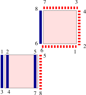
Figure 1: An $N=2$ loop configuration on a $2\times 2$ periodic lattice. The two plaquettes are shown separately for convenience. The numbers at the end of the dimers indicate connections. There are two loops in this configuration.

An update of the system involves flipping of a loop which means converting all solid dimers into dashed dimers within the loop and vice versa. Typically, a point is selected at random and the loop connected to it is flipped using a Metropolis decision. Since there are $(b+d)!/(d!b!)$ number of equivalent dimer configurations with $b$ solid and $d$ dashed dimers on a given bond, it is necessary to take this factor into account in the Metropolis decision to ensure detailed balance.

3 CHIRAL SUSCEPTIBILITY

To address the question of the existence of a massless pion in the chiral limit one can measure the chiral susceptibility $\chi$ as a function of the lattice size $L$. Since it is the first derivative of the chiral condensate with respect to the fermion mass it should diverge as a power of $L$ if there is a massless pion in the theory. For example if the chiral symmetry is spontaneously broken we must have $\chi\propto L^{d}$ where $d$ is the dimensions of the lattice. In the case of two dimensions where we expect chiral symmetry to remain unbroken, a massless pion leads to a divergence of the form $\chi\propto L^{(}2-\eta)$ where the KT prediction is that $0\leq\eta\leq 0.25$. Another example is the continuum two flavor Schwinger model where $\eta=1$.

To measure the chiral susceptibility, we introduce two monomers into each loop configuration in all possible ways. Since the loops are made up of an alternate sequence of solid and dashed bonds, introducing a monomer introduces a defect in the pattern. However, a single defect is impossible in a loop. Thus, in a two monomer configuration both monomers must be on the same loop. It is easy to see that a loop with two monomers can be generated by partially flipping a loop. Using this observation we find the chiral susceptibility by summing the weights of all the new configurations generated during the loop update. We have checked that our measurement of the susceptibility produces accurate answers on small lattices. Table 1, compares our results to exact calculations.

Table 1: Susceptibility: algorithm vs. exact results.

N	Lattice Size	Exact	Algorithm
1	$8\times 8$	5.27221…	5.2722(2)
2	$4\times 4$	6.40205…	6.402(2)
3	$4\times 4$	14.1595…	14.159(8)
5	$2\times 2$	9.57386…	9.574(7)
30	$2\times 2$	338.534…	338.2(8)

When we apply this algorithm to larger lattices we find that small clusters often get updated and occasionally even loops of large sizes get flipped. Our results for the chiral susceptibility for various lattice sizes is plotted in figure 2.

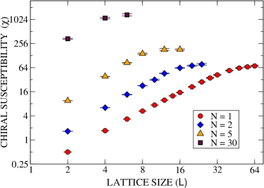
Figure 2: Chiral Susceptibility as a function of the lattice size $L$ for various values of $N$.

We can draw three conclusions from the plot. First, as a function of $L$ there is no evidence of a divergence for any $N$. Thus the pion is always massive. Second, since the value of $L$ where the susceptibility begins to level gives a rough indication of the inverse of the pion mass, the pion mass increases with $N$. Finally, the value of the chiral susceptibility diverges with $N$, signaling the formation of a condensate. However, our results suggest that this is not driven by long distance fluctuations.

Since the talk was given we have continued to study our algorithm more carefully. It now appears to us that there are configurations which we sample exponentially rarely as the volume increases but whose contribution is still finite to the final result. This problem begins to show up mildly around $L=32$ for $N=1$ through very large fluctuations. Of course we had collected very very large statistics to be able to control our error bars. However, we think the error analysis is not reliable since we may have uncontrolled auto-correlation times. For this reason we believe the error bars in figure 2 and in the graphs presented in [6] are incorrect. This also invalidates the conclusions made above and in [6]. Thus, although our representation is a useful first step and perhaps gives a qualitative picture for small volumes more work is needed before we can answer questions we raised in the first section.

References

- [1] N. Kawamoto and J. Smit, Nucl. Phys. B192, 100 (1981).
- [2] H. Kluberg-Stern, A. Morel, O. Napoly and B. Petersson, Nucl. Phys. B190, 504 (1981).
- [3] M. Salmhofer and E. Seiler, Comm. Math. Phys. 139, 395 (1991);ibid 146 637 (1992).
- [4] C. Gutsfeld, H. A. Kastrup and K. Stergio, Nucl. Phys. B560, 431 (1999).
- [5] P.Rossi and U. Wolff, Nucl. Phys. B248, 105 (1984).
- [6] S. Chandrasekharan, Phys. Lett. B536, 72 (2002).