Empirical Baye’s Method and Tests in Very Light Quark Range from The Overlap Lattice QCD

Abstract

Based on Bayesian theorem an empirical Baye’s method is discussed. A programming chart for mass spectrum fitting is suggested. A weakly constrained way for getting priors to solve the chiral log data fitting singularity is tested.

1 Introduction

Data analysis is an important procedure for most numerical projects and experiments. In lattice QCD, the theory we fit to hadronic two point correlation function is:

$$G(t,A,m) = \sum_{i=1}^{\infty}A_{i}e^{-m_{i}(t-t_{0})}$$ (1)

However, the general minimum $\chi^{2}$ procedure does not work for such a full physics hypothesis as the procedure is singular. What we used to do is to truncate both data set and theory. We might fit only the large-$t$ behavior with the lowest mass particle.

Numerically, the minimizing procedure is equivalent to a linear equation. Suppose ${\bf\rho}=\{A_{i},m_{i}\}$ is an unknown parameter vector

$${\rm minimize:}~{}~{}~{}\mathcal{A}({\bf\rho})$$ (2)

$$\Rightarrow \mid{\bf A\cdot\rho}-{\bf c}\mid=0$$

A singularity can occur due to the fact that matrix ${\bf A}$ has is degenerate or has zero eigenvalues. A possible solution to the singularity is to add another matrix ${\bf B}$. Suppose there is another minimizing procedure $\mathcal{B}({\bf\rho})$,

$$\mathcal{C}(\rho)=\mathcal{A}(\rho)+\lambda\mathcal{B}(\rho)$$

$$\Rightarrow \mid{\bf C\cdot\rho}-{\bf c}^{\prime}\mid=0$$

We can minimize $\mathcal{C}(\rho)$ instead of $\mathcal{A}(\rho)$.

2 Bayesian Theory

Bayesian statistics provides a useful way to offer such an additional minimizing procedure. The parameter vector $\rho$ describes the hypothesis of Eq. (1). To get $\rho$ from the measured data set $D$ is a numerical inverse problem. The Bayesian theorem tells us that [1]: a single good inverse ${\bf\rho}$, is to maximize the probability

$${\rm Prob}({\bf\rho}\mid{\bf D},\tilde{\rho})={\rm Prob}({\bf D}\mid{\bf\rho},\tilde{\rho})\cdot\frac{{\rm Prob}({\bf\rho}\mid\tilde{\rho})}{{\rm Prob}({\bf D}\mid\tilde{\rho})}$$ (4)

Here $\tilde{\rho}$ is a prior set of the hypothesis and ${\rm Prob}({\bf\rho}\mid\tilde{\rho})$ is the Bayesian prior probability.

Maximizing the entropy of $\rho$ under $\langle\rho\rangle=\tilde{\rho}$, $\langle\rho^{2}\rangle-\langle\rho\rangle^{2}=\tilde{\sigma}^{2}$ gives:

$${\rm Prob}(\rho\mid\tilde{\rho}) = \frac{1}{\sqrt{2\pi\tilde{\sigma}}}e^{-(\rho-\tilde{\rho})^{2}/2\tilde{\sigma}^{2}}$$

$${\rm Prob}(D\mid\rho,\tilde{\rho}) \propto e^{-\chi^{2}/2}$$

$$\chi_{prior}^{2} = \sum_{i}\frac{(\rho_{i}-\tilde{\rho}_{i})^{2}}{\tilde{\sigma}_{i}^{2}}$$ (5)

$$\Rightarrow\chi_{aug}^{2} = \chi^{2}+\chi_{prior}^{2}$$ (6)

So the Bayesian theorem tells us that a single good inverse $\rho$ is to minimize $\chi^{2}_{aug}$ [2][3]. Here the $\chi^{2}_{prior}$ plays the role of the additional minimizing term $\mathcal{B}(\rho)$ in Eq. (3) with $\lambda=1$.

3 Systematic errors and multiplier ${\bf\lambda}$

In principle, minimizing $\mathcal{A}(\rho)$ and minimizing $\mathcal{B}(\rho)$ would not necessarily give the same solution of $\rho$. Hereby, multiplier vector ${\bf\lambda}$ is a bridge from the solution of minimizing $\mathcal{A}$ to the solution of minimizing $\mathcal{B}$. With $\lambda=1$ the constrained data modeling always introduces some systematic bias which depends on how the input priors match the unknown hypothesis. In some of the cases if we know the physics very well, we can ”teach the physics in fitting procedure”. That means to input the priors according to our knowledge to the hypothesis [2]. However, in some of the cases we do not know the hypothesis well, only the measured data set $D$ can tell us the information both of the priors and hypothesis. We should not simply maximize the probability ${\rm Prob}(D\mid\tilde{\rho})$ to get the priors $\tilde{\rho}$, since that violates Bayesian theorem. Instead, we can consider to use a subset of the measured data. In Bayesian statistics when some data set $D_{1}$ comes along, and then some additional data set $D_{2}$ comes again, the probability of $\rho$ in these two cases will be [1]:

$${\rm Prob}(\rho\mid D_{1},\tilde{\rho})={\rm Prob}(\rho\mid\tilde{\rho})\cdot\frac{{\rm Prob}(D_{1}\mid\rho,\tilde{\rho})}{{\rm Prob}(D_{1}\mid\tilde{\rho})}$$

$${\rm Prob}(\rho\mid D_{2},\tilde{\rho})={\rm Prob}(\rho\mid\tilde{\rho})\cdot\frac{{\rm Prob}(D_{2}\mid\rho,\tilde{\rho})}{{\rm Prob}(D_{2}\mid\tilde{\rho})}$$ (7)

One can then prove the estimate of $\rho$ probability in a enlarged data set:

$${\rm Prob}(\rho\mid D_{2}D_{1},\tilde{\rho})$$ (8)

$$= {\rm Prob}(\rho\mid\tilde{\rho})\cdot\frac{{\rm Prob}(D_{2}D_{1}\mid\rho,\tilde{\rho})}{{\rm Prob}(D_{2}D_{1}\mid\tilde{\rho})},$$

which shows that we would have the same answer if all the data $D_{1}D_{2}$ had been taken together. Furthermore, we can get the priors from data set $D_{1}$ then to fit $\rho$ from $D_{1}D_{2}$ taken together. That will not violate the Bayesian theorem. So we can construct a real empirical Baye’s method to make data modeling. All the information comes from measured data set, without any additional artificial bias. For example, we can give a programming chart for the mass spectrum fitting such as in Fig. 1.

Figure 1: A programming chart of the empirical Baye’s method. Where $I\neq 0$, $M\neq 0$, $N$ is the number of the parameters in each fitting procedure, $N_{max}$ is the maximum number of the parameters we want to fit, $D$ is the number of the data points we use to fit the parameters, $\lambda_{i}$ is $i_{th}$ element of the multiple vector ${\bf\lambda}$

We test this empirical Baye’s method on a $16^{3}\times 28$ lattice, with $\beta=2.264$ Iwasaki gauge action. Quenched approximation with anti-periodic boundary in t-direction is used. $f_{\pi}$ scale gives $a^{-1}=0.9775(47)$GeV. The lowest pion mass is about $m_{\pi}\approx 179$MeV, $m_{\pi}/m_{\rho}\approx 0.25$. Empirical Baye’s method works in such light quark area. Fig. 2 shows the $\lambda$ test at $m_{\pi}\approx 202$MeV. Where whole elements of vector $\lambda$ are equal to 1, except the first and second elements $\lambda_{1},~{}\lambda_{2}$ are varying and $\lambda_{1}=\lambda_{2}$. This test shows that the pion mass is stable, the priors were obtained from data subset matches full data set very well [4].

An other advantage of this empirical Baye’s method is that sometimes we can observe a stable excited state. Fig. 3 shows the nucleon mass and the mass of the first excited state. The mass ratio shows that the excited state is consistent with the nucleon Roper state which lattice community has searched for years but have not been successful before[5].

$$\frac{m_{\rm exc}}{m_{N}}\sim 1.54\pm 0.17$$

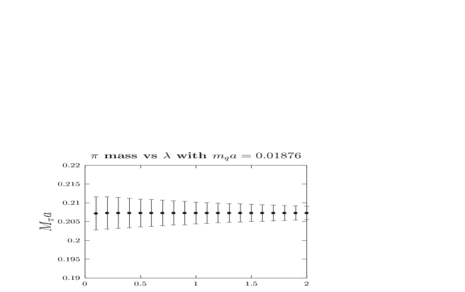
Figure 2: The $\lambda$ test for pion mass at $m_{\pi}\approx 202$MeV

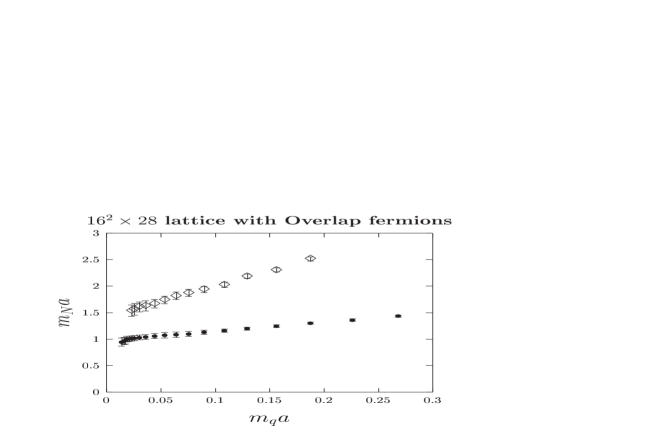
Figure 3: The Roper state as an excited state of the nucleon

4 Quenched chiral log fitting and the weak prior method

The quenched chiral log is a hard problem, since the general minimum $\chi^{2}$ data modeling for the chiral log formula is singular [6][4]. The normal equation in the fitting procedure gives only 2 independent parameters, the third one is not independent.

$$m^{2}_{PS}=2Am_{q}\{1-\delta[\ln(2Am_{q}/\Lambda^{2}_{\chi})+1]\}+O(m_{q}^{2})$$ (9)

An additional matrix is really needed to lift the degeneracy in order to get the priors from data. An alternative way is to use weak constrained data modeling to get the good priors. In this case we input $\delta=0.20\pm 0.20,~{}\Lambda_{\chi}=1.1\pm 0.5$ as the weak priors. From a data subset of $m_{\pi}=179$MeV to $m_{\pi}=287$MeV to get the better priors. We then input this better priors into the full data set of $m_{\pi}=179$MeV to $m_{\pi}=312$MeV, and obtain $\delta=0.26\pm 0.03$, $\Lambda=1.1\pm 0.1$GeV. Fig. 4 shows the resultant fit of $(m_{\pi}a)^{2}$.

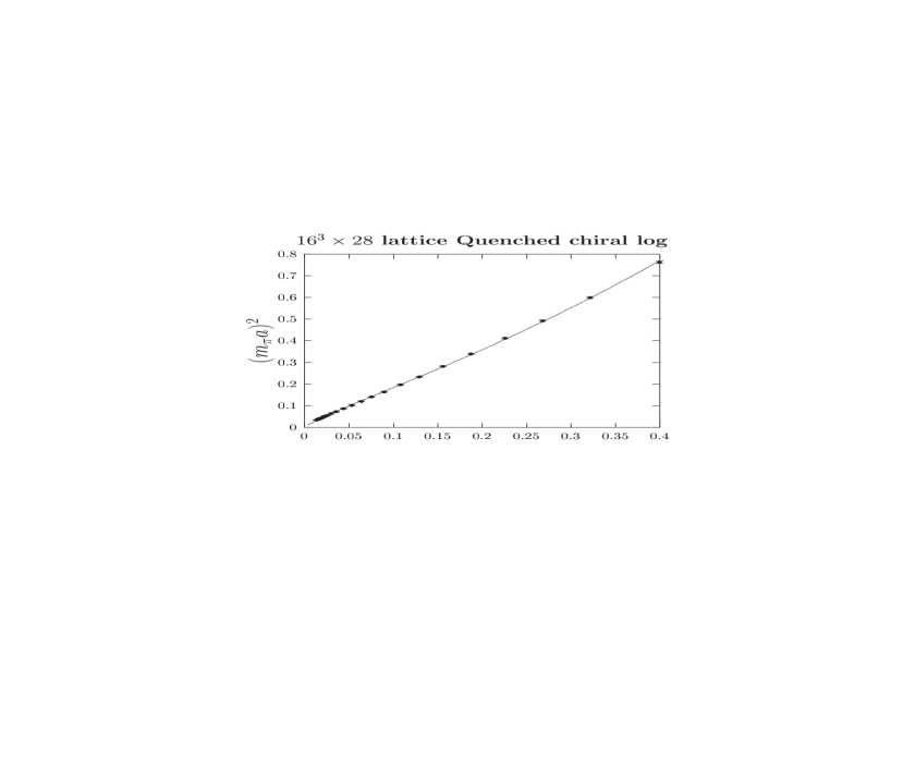
Figure 4: The weak constrained data modeling for the quenched chiral log

Further work is on the way to improve the stability of the fitting program, especially in the very light quark region, and try to automate the procedure.

References

[1] S.J. Press, Bayesian Statistics: Principles, Models and
Applications, (Wiley, New York, 1989).
[2] G. P. Lepage, et al., Nucl.Phys.B(Proc. Suppl.) 106(2002)12
hep-lat/0110175.
[3] C. Morningstar, hep-lat/0112023.
[4] T. Draper et al., Proceeding of Lattice 2002 hep-lat/0208045,
S.J. Dong et.al., Nucl. Phys. B (Proc. Suppl.) 106 (2002) 275.
[5] F.X. Lee et al., Proceeding of Lattice 2002 hep-lat/0208070,
Frank X. Lee et al., Nucl. Phys. B (Proc. Suppl) 106 (2002) 248.
[6] CP-PACS Collaboration, Phys. Rev. Lett. 84 (2000) 238.