Abstract

I present a selection of CP-PACS and UKQCD data for the pseudo-Goldstone masses in $N_{f}\!=\!2$ QCD with doubly degenerate quarks. At least the more chiral points should be consistent with Chiral Perturbation Theory for the latter to be useful in an extrapolation to physical masses. I find consistency with the chiral prediction but no striking evidence for chiral logs. Nonetheless, the consistency guarantees that the original estimate, by Gasser and Leutwyler, of the $N_{f}\!=\!2$ QCD low-energy scale $\Lambda_{3}$ was not entirely wrong.

Introduction

Ever since numerical lattice QCD computations have been done, the spectrum of light mesons has served as a benchmark problem. This is still true today, as actions respecting the global chiral symmetry among the light flavours are being tested and several groups have embarked on ambitious simulations of “full” QCD with two or possibly more dynamical flavours. These developments address one of the key issues in low-energy QCD. The fact that chiral symmetry is both spontaneously and explicitly broken generates pseudo-Goldstone bosons, i.e. particles that dominate (for small enough quark masses) the long-range behaviour of correlators between external currents and which are collectively called “pions”.

The lattice is not the only framework to address the low-energy structure of QCD. In the old days PCAC relations were exploited to predict the dependence of low-energy observables on shifts in the quark masses and external momenta. The one best known is

$$F_{\pi}^{2}M_{\pi}^{2}=(m_{\mathrm{u}}\!+\!m_{\mathrm{d}})\;|\langle 0|\bar{q}q|0\rangle|+O(m^{2})$$ (1)

which connects the pion mass and decay constant to the product of the explicit and spontaneous symmetry breaking parameters. However, the Gell-Mann – Oakes – Renner relation (1) does not give a prediction how $F_{\pi}$ and $M_{\pi}$ separately depend on the quark mass. And in the real world the latter may be shifted only by a discrete amount (e.g. by replacing $d\to s,\pi\to K$ one gets a leading order prediction for the quark mass ratio $m_{s}/m$ with $m\equiv(m_{u}\!+\!m_{d})/2$).

Today, the first limitation is overcome, since the successor of PCAC, Chiral Perturbation Theory [1], gives detailed predictions how either $M_{\pi}$ or $F_{\pi}$ individually depends on the quark mass $m$. And – in principle – the second problem is gone since one may vary $m$ continuously in a lattice computation. Therefore, it seems natural to combine the two approaches to benefit from their respective advantages. However, for that aim quarks need to be taken sufficiently light, and this is a numerical challenge on the lattice. Below, an elementary test is presented whether this is already achieved in present state-of-the-art results for $M_{\pi}^{2}$ versus $m$, as published by the CP-PACS [2] and UKQCD [3] collaborations. The idea is to restrict the analysis to the “doubly degenerate” case with $N_{\!f\,}\!=\!2$ $O(a)$ improved Wilson quarks, i.e. to consider only the subset where both valence-quarks are exactly degenerate with the sea-quarks, as this avoids additional assumptions of the “partially quenched” framework.

Prediction by Chiral Perturbation Theory

Here, I give a brief summary of the work by Gasser and Leutwyler (GL), with an application to lattice data in mind.

GL have calculated the substitute for the GOR relation (1) to NLO in Chiral Perturbation Theory (XPT) with $N_{\!f\,}\!=\!2$ quarks [1]. To that order, two low-energy constants from the LO Lagrangian appear ($F\!=\!\lim_{m\to 0}F_{\pi},B\!=\!-\lim_{m\to 0}\langle 0|\bar{q}q|0\rangle/F^{2}$) together with the finite parts of the $l_{i}$ in the NLO Lagrangian. Restricted to the degenerate case their result [1] takes the form

$$M_{\pi}^{2}\! \!=\! \!M^{2}+{1\over F^{2}}\Big{(}{M^{4}\over 32\pi^{2}}\log({M^{2}\over\mu^{2}})-2M^{4}\,l_{3}^{\mathrm{r}}(\mu)\Big{)}$$ (3)

$$F_{\pi}\! \!=\! \!F+{1\over F}\Big{(}-\!{M^{2}\over 16\pi^{2}}\log({M^{2}\over\mu^{2}})+M^{2}\,l_{4}^{\mathrm{r}}(\mu)\Big{)}$$ (4)

$$M^{2}\! \!\equiv\! \!2mB\;.$$ (5)

Note that (3, 4) has the typical structure of a NLO prediction: A chiral logarithm summarizing the contribution from the pion loops appears together with a counterterm. The $l_{i}^{\mathrm{r}}$ are the renormalized GL coefficients, i.e. they are the descendents of the $l_{i}$ which appear in the NLO Lagrangian and which are divergent quantities. As a result, the $l_{i}^{\mathrm{r}}$ depend on the (chiral) renormalization scale $\mu$. In the dimensionally regularized theory one has [1]

$$l_{i}\! \!=\! \!l_{i}^{\mathrm{r}}(\mu)+\gamma_{i}\lambda(\mu)$$ (6)

$$\lambda(\mu)\! \!=\! \!{-1\over 16\pi^{2}\mu^{4-d}}\Big{(}{1\over 4-d}+{\log(4\pi)+\Gamma^{\prime}(1)+1\over 2}\Big{)}$$ (7)

$$l_{i}^{\mathrm{r}}(\mu)\! \!=\! \!l_{i}^{\mathrm{r}}(\mu^{\star})-{\gamma_{i}\over 16\pi^{2}}\log({\mu\over\mu^{\star}})$$ (8)

and the $\beta$-function coefficients $\gamma_{i}$ are known. In the present context only $\gamma_{3}=-{1\over 2}\,,\;\gamma_{4}=2$ [1] are relevant, and this suggests that one rewrites (3, 4) with the help of

$$l_{i}^{\mathrm{r}}={\gamma_{i}\over 32\pi^{2}}\Big{(}\bar{l}_{i}+\log({M^{2}\over\mu^{2}})\Big{)}\;,$$ (9)

where the $\mu$ dependence in $l_{i}^{\mathrm{r}}\!=\!l_{i}^{\mathrm{r}}(\mu)$ is traded for an $M$ dependence in $\bar{l}_{i}\!=\!\bar{l}_{i}(M)$, to get [1]

$$M_{\pi}^{2}\! \!=\! \!M^{2}\,\Big{(}1-{M^{2}\over 32\pi^{2}F^{2}}\bar{l}_{3}+O(M^{4})\Big{)}$$ (10)

$$F_{\pi}\! \!=\! \!F\;\Big{(}1+{M^{2}\over 16\pi^{2}F^{2}}\bar{l}_{4}+O(M^{4})\Big{)}\;.$$ (11)

The NLO part is given in terms of the LO parameters $F,B$ and the NLO coefficients $\bar{l}_{3},\bar{l}_{4}$. While the former two are known quite accurately, for the $\bar{l}_{i}$ only their running in $M^{2}$ is known exactly and the phenomenological estimate of the integration constants has comparatively large error-bars. Gasser and Leutwyler give in their initial paper [1] the estimate

$$\bar{l}_{3}(m_{\mathrm{phys}})=2.9\pm 2.4\;,\qquad\bar{l}_{4}(m_{\mathrm{phys}})=4.3\pm 0.9$$ (12)

for real world quark masses. It turns out that even this limited information is useful, since it determines the curvature of $M_{\pi}$ as a function of the quark mass. Close to the chiral limit, both $\bar{l}_{i}$ are positive and as a consequence $M_{\pi}^{2}$ does not rise strictly linear in $m$ but turns right, while $F_{\pi}$ has a positive first derivative in $m$. More specifically, (12) translates into

$$M_{\pi,\mathrm{phys}}\!\simeq\!139\,\mathrm{MeV}\,,\;F_{\pi,\mathrm{phys}}\!\simeq\!92.4\,\mathrm{MeV}\;\Longleftrightarrow\;M_{\mathrm{phys}}\!\simeq\!141\,\mathrm{MeV}\,,\;F\!\simeq\!86.1\,\mathrm{MeV}$$ (13)

which means that the physical pion is somewhat lighter than it would be, if the LO relation were exact, while is decay constant exceeds its value in the chiral limit by $\sim\!7\%$.

A seemingly formal point which, in the end, proves convenient in analyzing the lattice data is the following. A naive look at (10) suggests that the typical structure of a NLO prediction is gone – rather than a $M^{4}$ and a $M^{4}\log(M^{2})$ contribution, only the polynomial part seems left. The point is that this impression is entirely misleading; the IR divergencies (which are genuine to QCD in the chiral limit) are not gone, they are just hidden in the $\bar{l}_{i}$. The situation is, in fact, opposite – the $M^{4}$ part has been eliminated in favour of a pure $M^{4}\log(M^{2})$ contribution, and the last step is to make this apparent. The quark mass dependence of $\bar{l}_{3}$ is given through

$$\log({\Lambda_{i}^{2}\over M^{2}})=\log({\Lambda_{i}^{2}\over M_{\mathrm{phys}}^{2}})+\log({M_{\mathrm{phys}}^{2}\over M^{2}})=\bar{l}_{i}(m_{\mathrm{phys}})+\log({M_{\mathrm{phys}}^{2}\over M^{2}})=\bar{l}_{i}(m)$$ (14)

and together with (5), the relation takes its final form (see e.g. [4])

$$M_{\pi}^{2}\! \!=\! \!2mB-{m^{2}B^{2}\over 8\pi^{2}F^{2}}\log({\Lambda_{3}^{2}\over 2mB})+O(m^{3})$$ (15)

$$F_{\pi}\! \!=\! \!F+{mB\over 8\pi^{2}F}\log({\Lambda_{4}^{2}\over 2mB})+O(m^{3})$$ (16)

where $\Lambda_{4},\Lambda_{3}$ represent universal low energy scales. The estimates (12) translate into

$$\Lambda_{3}=0.6\,\mathrm{GeV}\begin{tabular}[]{l}$+1.4\,\mathrm{GeV}$\\ $-0.4\,\mathrm{GeV}$\end{tabular}\;,\qquad\Lambda_{4}=1.2\,\mathrm{GeV}\begin{tabular}[]{l}$+0.7\,\mathrm{GeV}$\\ $-0.4\,\mathrm{GeV}$\end{tabular}\;.$$ (17)

It is worth emphasizing that all four parameters $F,M^{2}\!=\!2Bm,\Lambda_{3},\Lambda_{4}$ do not depend on the QCD renormalization scheme [1], i.e. they are the proper physical low-energy parameters at order $O(p^{4})$. Furthermore the $\Lambda_{i}$ do not depend on the quark masses, and this means that the representation (15, 16) is perfectly suited to analyze the lattice data even if they are gotten at quark masses larger than $m\equiv(m_{\mathrm{u}}\!+\!m_{\mathrm{d}})/2$ in the real world – as long as they are not beyond the regime of validity of the chiral expansion itself.

The latter point is one of the key issues in the comparison we aim at. The chiral expansion is known to be asymptotic, and this means that increasing the order will enhance the accuracy near the chiral limit – at the price of worsening the prediction for heavier masses. What is the “critical scale” beyond which the chiral expansion “explodes” is, a priori, not known. From a formal point of view, one might think that (10, 11) indicate that the expansion is in $M/(4\pi F)$ and hence hope that it is good for pion masses up to $1\,\mathrm{GeV}$. In this paper I will argue that watching the convergence pattern at a fixed quark mass gives a more reliable estimate what is the permissible range. This is facilitated since the NNLO expression for $M_{\pi}^{2}$ (with $N_{\!f\,}\!=\!2$) is known [5, 6]. The result reads (for the presentation I follow [4])

$$M_{\pi}^{2}=2mB\bigg{(}1-{mB\over 16\pi^{2}F^{2}}\log({\Lambda_{3}^{2}\over M^{2}})+{m^{2}B^{2}\over 64\pi^{4}F^{4}}\Big{\{}{17\over 8}\Big{(}\log({\Lambda_{M}^{2}\over M^{2}})\Big{)}^{2}+k_{M}\Big{\}}+O(m^{3})\bigg{)}$$ (18)

where $\Lambda_{M}$ is implicitly defined through $51\log({\Lambda_{M}^{2}\over\mu^{2}})=28\log({\Lambda_{1}^{2}\over\mu^{2}})+32\log({\Lambda_{2}^{2}\over\mu^{2}})-9\log({\Lambda_{3}^{2}\over\mu^{2}})+49$ and the mass-independent $k_{M}$ accounts for the remainder at $O(p^{6})$, in particular the new counterterms. Phenomenological values for $\Lambda_{M}$ and $k_{M}$ will be mentioned below.

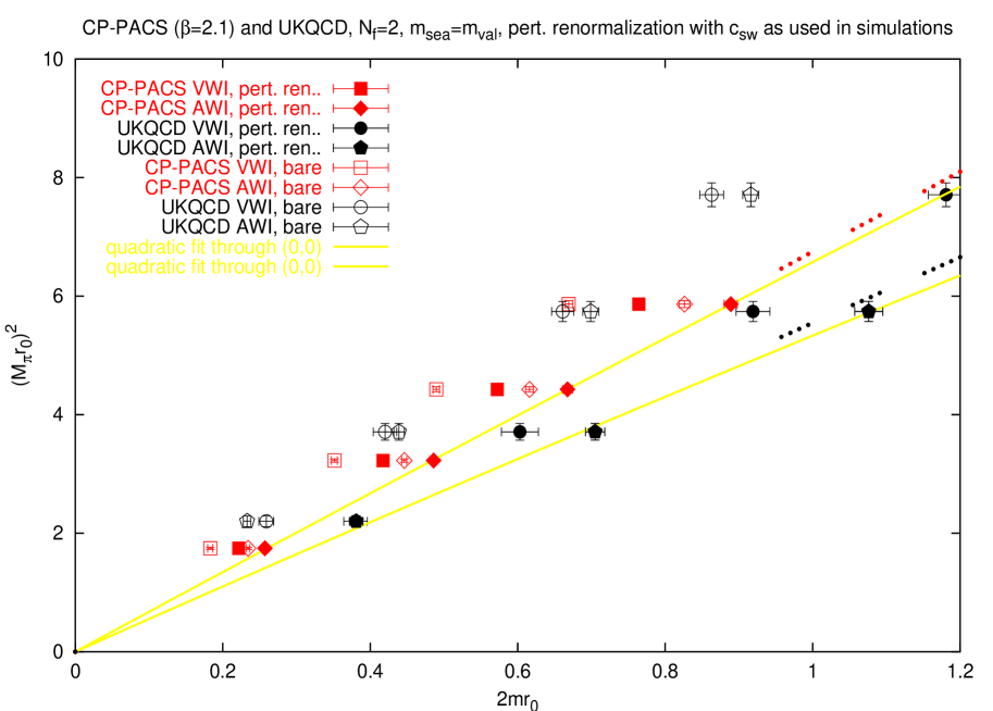
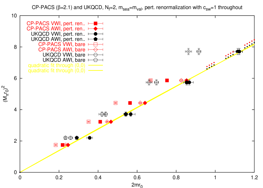
Figure 1: CP-PACS and UKQCD data converted to the form $M_{\pi}^{2}$ vs. $2m$ with masses in units of $r_{0}^{-1}$. Top: Perturbative renormalization with $c_{\mathrm{SW}}$ as used in the simulations. Bottom: Same but $c_{\mathrm{SW}}=1$ throughout. A quadratic fit, constrained to go through zero, is applied to the renormalized AWI data. Segments of the asymptotic slope in the chiral limit highlight the curvature.

Lattice Data

We are now in a position to esteem the results by the CP-PACS and UKQCD collaborations for the quark mass dependence of the pion mass. We shall consider, out of these $N_{\!f\,}\!=\!2$ data, only the two-fold degenerate case where both valence quarks have the same mass and where they are, at the same time, exactly degenerate with the sea quarks so that the theory is unitary.

The CP-PACS collaboration has simulated various ($\beta,\kappa$) combinations with an RG improved gauge action and a mean-field improved clover quark action [2]. They use a grid of size $12^{3}\!\times\!24,16^{3}\!\times\!32,24^{3}\!\times\!48,24^{3}\!\times\!48$ at $\beta\!=\!1.8,1.95,2.1,2.2$, respectively, which leads to a lattice spacing, if determined through the $\rho$ mass, between $0.215\,\mathrm{fm}$ and $0.087\,\mathrm{fm}$ and hence a spatial box size between $2.58\,\mathrm{fm}$ and $2.08\,\mathrm{fm}$. With so much information at hand, one could, in principle, attempt a continuum extrapolation for $M_{\pi}^{2}$ versus the sum of the (degenerate) quark masses, $2m$. However, non-perturbative renormalization might be necessary, and/or the lattice spacing might be too large at the lower $\beta$ values. For this reason, I have decided to concentrate on the $\beta\!=\!2.1$ data, since here discretization effects are not supposed to be too large, and good statistics is available. At that $\beta$ value, even the lightest pion is unlikely to suffer from finite-size effects, since $M_{\pi}L\!>\!7$, and the lattice spacing determined via the $\rho$ mass is of order $0.1\,\mathrm{fm}$ and hence comparable with that in the UKQCD simulations.

The UKQCD collaboration works on a $16^{3}\times 32$ grid, using different actions: Wilson glue and non-perturbatively $O(a)$ improved clover quarks [3]. Another point in which they differ from CP-PACS is a tactical one: they try to relax $\beta$ in pushing $\kappa_{\mathrm{sea}}$ up (i.e. the quark mass down) such that the lattice spacing, in units of $r_{0}$, stays constant. Numerically, it is $a\!\sim\!0.1\,\mathrm{fm}$ for the data considered below (though the ensemble at $(\beta,\kappa_{\mathrm{sea}})\!=\!(5.2,0.1355)$ is not matched any more), and the hope is that the size of discretization effects would be approximately constant. This choice implies that the physical box size stays constant, too, and the bound $M_{\pi}L\!>\!4.5$ maintained makes one feel comfortable that finite size effects are small.

The plan of this article is to ignore that the dynamical quark masses might be too heavy for the chiral prediction to be applicable and to ignore that in principle a continuum extrapolation is needed but instead to go ahead and simply compare the two datasets on a “as-is” basis with the LO/NLO/NNLO prediction from Chiral Perturbation Theory in the continuum. With the relevant low-energy constants on the chiral side given in physical units, $r_{0}^{-1}$ must be so, too. In this article, this is done through the assumption that $r_{0}^{-1}$ represents a universal low-energy scale, unaffected by unquenching effects; the numerical value used is $r_{0}\!=\!0.5\,\mathrm{fm}$ [7].

On the lattice, there are two definitions of the “quark mass”, one through the vector Ward-Takahashi identity (VWI mass), one through the axial identity (AWI mass). The bare masses (open symbols in Fig. 1) need not agree, while after renormalization (filled symbols in Fig. 1) they would (up to $O(a^{2})$ effects) if the renormalization factors were computed non-perturbatively. For unquenched ($N_{\!f\,}\!=\!2$) data the relevant non-perturbative factors are not yet available. For this reason, I have decided to renormalize both the CP-PACS and the UKQCD data at one-loop order (the details being given in the appendices). In the case of the CP-PACS data this basically repeats their calculation [2], albeit with two notable differences: First, the scale is set through the measured $r_{0}$, since this is the only possibility with the UKQCD data. Second, the “boost factor” $u_{0}$ is derived from the measured plaquette rather than the plaquette in the chiral limit, since in the UKQCD data there is no uniquely defined chirally extrapolated version. This perturbative calculation then lays the ground on which the CP-PACS and UKQCD data may be compared to each other and to the chiral prediction.

Fig. 1 displays $(M_{\pi}r_{0})^{2}$ versus the renormalized quark masses with filled symbols, open symbols indicate the bare data to visualize the shift. In the upper part the renormalization was performed with the $c_{\mathrm{SW}}$ values as they were used in the simulations (suggested by a mean-field analysis [2] or the Alpha study [3, 8]). In the lower part the renormalization factors were computed with $c_{\mathrm{SW}}\!=\!1$ throughout, which is a consistent choice at one-loop order. Obviously, the overall consistency of the data is much better with this latter choice, as is particularly obvious from the quadratic fits (constrained to go through zero) to the AWI data. Henceforth, we shall stick to the latter choice ($c_{\mathrm{SW}}\!=\!1$), but it is useful to keep in mind that the difference to the upper part is a clear indication of the size of inherent perturbative uncertainties. Finally, it is worth mentioning that all error-bars in this article represent only statistical errors.

We now turn to the physics content. To convey a feeling for the scales, I mention that at $2mr_{0}\!=\!1$ the sum of the valence quark masses is of order $400\,\mathrm{MeV}$, i.e. about four times as much as in a physical $K$, and the corresponding “pion” weighs about $1\,\mathrm{GeV}$. The physical kaon weighs $496\,\mathrm{MeV}$, i.e. $(M_{K}r_{0})^{2}\!\simeq\!1.58$. If the pion would satisfy $(M_{\pi}r_{0})^{2}\!\simeq\!1.58$ this would mean that its $u$- and $d$-quarks are about half as heavy as the $s$-quark in the real world. The lightest pion in the CP-PACS and UKQCD simulations have $(M_{\pi}r_{0})^{2}$ values 1.75 and 2.20, respectively, and from this we conclude that their lightest $u$- and $d$- quarks (in the unitary theory) have about 55% and 70% of the mass of the physical strange quark.

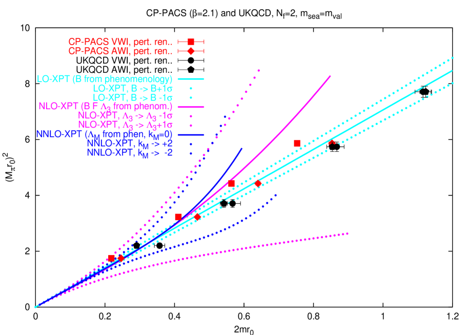
Figure 2: LO/NLO/NNLO chiral predictions with phenomenological values for $B,F,\Lambda_{3},\Lambda_{M},k_{M}$ $(\pm 1\sigma$ variation included at each order, cf. text for details$)$ compared to the renormalized data in the version with $c_{\mathrm{SW}}=1$. Note that the lines represent parameter-free predictions, not fits.

With such heavy “light” quarks it is a priori not clear whether XPT is of any use to extrapolate them to the physical $u$- and $d$-quark masses. In an attempt to shed a light on this issue, Fig. 2 shows the renormalized data (as in the bottom part of Fig. 1) together with the predictions from XPT at tree/one-loop/two-loop level (LO/NLO/NNLO). The low-energy constants are taken from phenomenology, i.e. these curves represent parameter-free predictions. At LO the chiral prediction is a straight line with the slope parameter $B$ taken from (2); the $\pm 1\sigma$ bounds are indicated by dotted lines. At NLO the prediction is curved, and the numerical values of the additional parameters are taken from (13) and (17). $\Lambda_{3}$ is varied within its phenomenological $\pm 1\sigma$ bound (full versus dotted lines – lowering $\Lambda_{3}$ to $200\,\mathrm{MeV}$ yields the upper, increasing it to $2\,\mathrm{GeV}$ yields the lower dotted line), with $B,F$ fixed at their central values. At NNLO the parameters $\Lambda_{M},k_{M}$ in (18) are determined as follows. With $\Lambda_{1}\!=\!0.11\!\pm\!{0.04\atop 0.03}\,\mathrm{GeV},\Lambda_{2}\!=\!1.2\!\pm\!0.06\,\mathrm{GeV}$ [9] and (17) the relation beneath eqn. (18) gives

$$\Lambda_{M}=0.60\!\pm\!0.03\,\mathrm{GeV}$$ (19)

where errors have been added in quadrature. This means that over the range considered the uncertainty in $\Lambda_{M}$ is neglibigle compared to that coming from $k_{M}$. Phenomenological arguments indicate $|k_{M}|\!\sim\!2$ [10], and the sum-rule estimates for the NNLO counterterms given in [9] may be converted into a more accurate estimate. For the purpose of the present article it is sufficient to use $k_{M}\!=\!0\pm 2$, and the associate curves (holding $B,F,\Lambda_{3},\Lambda_{M}$ fixed at their central values) are included in Fig. 2.

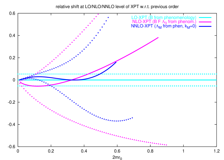
Figure 3: Relative shifts in $M_{\pi}^{2}$ versus $2mr_{0}$ in XPT – due to the uncertainty in $B$ at LO (light), due to NLO contribution with $B$ fixed at central value, $\Lambda_{3}$ varied within $1\sigma$ bound (intermediate), and due to NNLO contribution with $B$ and $\Lambda_{3}$ fixed at central values, $k_{M}\in\{0,\pm 2\}$ (dark).

This information is sufficient to asses the chiral convergence behaviour in $M_{\pi}^{2}$ versus $2m$. To that aim we compare the LO/NLO/NNLO predictions for a given quark mass. Fig. 3 shows the relative shift in $M_{\pi}^{2}$ when one more order is included or the new low-energy constants are varied within reasonable bounds. At first sight, the uncertainties at higher orders due to the error bars of the counterterms seem large, but one should keep in mind that the associate shifts are 100% correlated over the whole range. For instance, if the CP-PACS VWI point at $2mr_{0}\!\sim\!0.2$ sits on the $-1\sigma$ curve (upper dotted NLO line in Fig. 2), then the one at $2mr_{0}\!\sim\!0.4$ should too, if only $\Lambda_{3}$ needs to be adapted. This means that precise lattice data are ideally suited to reduce the error on $l_{3}^{\mathrm{r}}(\mu)$ (or $\Lambda_{3}$). Fig. 3 shows that the crossover where the uncertainty due to the NLO exceeds that due to the LO contribution is at $2mr_{0}=0.45/0.02/0.10$ when $\Lambda_{3}$ is taken at its central/+1$\sigma$/-1$\sigma$ value. By averaging with weights 2/1/1 one arrives at the estimate that in the case of $M_{\pi}$ the chiral expansion is sufficiently well-behaved that the NLO functional form is useful for quark masses up to

$$2mr_{0}\leq 0.25\qquad\Longleftrightarrow\qquad(M_{\pi}r_{0})^{2}\leq 2\qquad\Longleftrightarrow\qquad M_{\pi}\leq 560\,\mathrm{MeV}\;,$$ (20)

and maybe more. This, if correct, means that current state-of-the-art simulations make contact with the regime where NLO-XPT holds, but so far a non-trivial “lever arm” which is needed to make model independent predictions in the deeply chiral regime, is likely missing.

While it is clear that future simulation data will allow to test the prediction (20) and provide, if it is correct, the lever arm needed, one might, already at this time, go ahead and try what comes out if one assumes that the estimate (20) is too pessimistic and hence uses the NLO chiral ansatz to fit the data over an extended range. This is what we shall do below, but it is clear that this attempt is rather speculative and results should be taken with care.

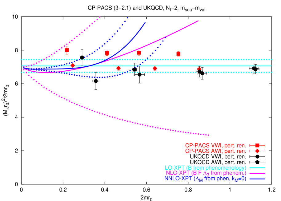
Figure 4: Same as Fig. 2, after dividing by $2mr_{0}$. Still, lines represent parameter-free chiral predictions at LO/NLO/NNLO (from light to dark colour), not fits.

Since everything below is about the deviation from a linear relationship, it is useful to make the curvature optically visible. This is conveniently done by dividing out a factor $2mr_{0}$. The result is displayed in Fig. 4 where the predictions from XPT at LO/NLO/NNLO are included for completeness. In this representation, the genuine feature of the NLO curve is that it lies below the LO constant for light pions, but above if the (LO-) pion mass is larger than $\Lambda_{3}$.

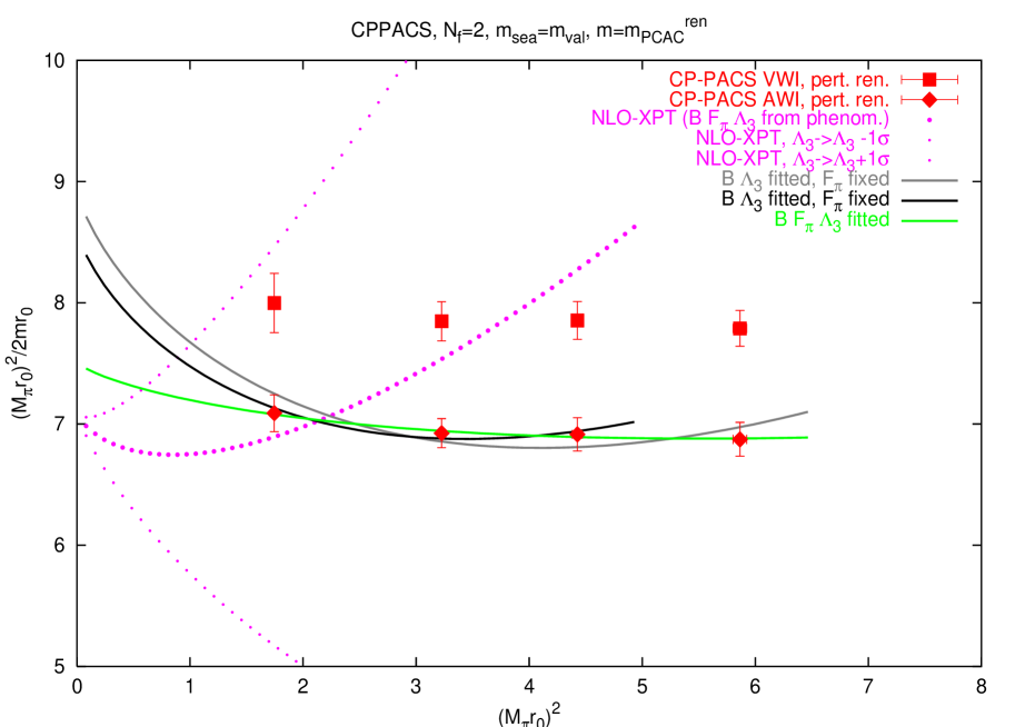
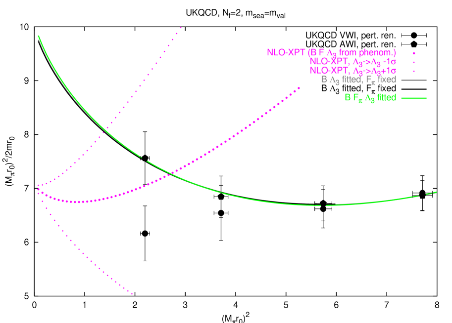
Figure 5: Fits of the data with the AWI quark mass to the NLO functional form (together with the allowed band from phenomenological estimate of $\Lambda_{3}$). In spite of the bound (20) being ignored, the data fit well to the suggested form (even if one insists on the phenomenological value of $F_{\pi}$ in the NLO ansatz (15, 21)), but with the current error-bars the LO functional form is still appropriate.

To fit the data, one replaces $2mB$ by $M_{\pi}^{2}$, since in this form the data are plotted against something which is directly measured and the change is of yet higher order in the chiral counting. In other words, the statement is that one should use the representation

$${\tilde{M}_{\pi}^{2}\over 2\tilde{m}}=\tilde{B}\,\Big{\{}1-{\tilde{M}_{\pi}^{2}\over 32\pi^{2}\tilde{F}_{\pi}^{2}}\log\Big{(}{\tilde{\Lambda}_{3}^{2}\over\tilde{M}_{\pi}^{2}}\Big{)}\Big{\}}$$ (21)

and adjust the 3 dimensionless parameters $\tilde{B}\!\equiv\!Br_{0},\tilde{F}\!\equiv\!F_{\pi}r_{0},\tilde{\Lambda}_{3}\!\equiv\!\Lambda_{3}r_{0}$.

	$Br_{0}$	$F_{\pi}r_{0}$	$\Lambda_{3}r_{0}$	$\chi^{2}/\mathrm{d.o.f.}$	$Br_{0}$	$F_{\pi}r_{0}$	$\Lambda_{3}r_{0}$	$\chi^{2}/\mathrm{d.o.f.}$
phenom. [1, 2]	7.09	0.234	1.52	—	7.09	0.234	1.52	—
CP-PACS-a	10.1	(0.234)	3.32	2.63/2	8.92	(0.234)	3.34	1.67/2
CP-PACS-b	9.65	(0.234)	3.01	0.23/1	8.58	(0.234)	3.06	0.16/1
CP-PACS-c	8.30	0.577	4.16	0.08/1	7.50	0.458	3.87	0.04/1
CP-PACS-LO	7.85	—	—	0.61/3	6.93	—	—	0.67/3
UKQCD-a	8.05	(0.234)	3.21	0.73/2	10.0	(0.234)	3.95	0.04/2
UKQCD-b	7.62	(0.234)	2.89	0.32/1	9.97	(0.234)	3.93	0.04/1
UKQCD-c	5.98	?	?	0.09/1	10.1	0.231	3.94	0.04/1
UKQCD-LO	6.67	—	—	1.39/3	6.90	—	—	1.51/3

Table 1: Coefficients in the fits of the NLO functional form $(\ref{Mpifit})$ to the degenerate CP-PACS and UKQCD data with VWI (left) or AWI (right) definition of the quark masses, after 1-loop renormalization as detailed in the appendix. Phenomenological values for comparison; constrained values in brackets. In one case, there is such a shallow minimum that the fitting algorithm fails to determine it. In general, $\chi^{2}$ is underestimated, since the fact that errors are correlated has been ignored. Since the main uncertainty is systematic, I refrain from quoting statistical errors.

Attempts to fit the data with either the VWI or the AWI definition of the quark mass to formula (21) are summarized in Tab. 1 and – for the AWI mass – illustrated in Fig. 5. Since the parameter $\tilde{F}_{\pi}\!=\!F_{\pi}r_{0}\!=\!92.4\,\mathrm{MeV}\,0.5\,\mathrm{fm}\!\simeq\!0.234$ is known, it is held fixed at its physical value in (a, b) and fitted only in case (c). Fit (b) differs from (a) in that the data point with the heaviest quark mass has been omitted. From the overall spread it is clear that there are considerable systematic uncertainties and this is why I refrain from quoting statistical errors.

It is clear that with the quality of the present data one cannot claim direct evidence for chiral logs. Nonetheless, it is worth noticing that fits (a) and (b) indicate that the data are consistent with the logarithmic form (21) suggested by NLO chiral perturbation theory. Moreover, that the fit with $F_{\pi}$ held fixed at its physical value does not dramatically change if the heaviest data point is omitted (a$\to$b), suggests that the estimate (20) for the permissible range at NLO level is indeed reasonable. What one can learn from Table 1 is that in QCD with $N_{\!f\,}\!=\!2$ the low-energy parameter $\Lambda_{3}$ does not differ by orders of magnitude from the original estimate by Gasser and Leutwyler [1]; all $\Lambda_{3}$ values in Tab. 1 lie between the central and the $+1\sigma$ level in (12). This is important, since it excludes – at least for $N_{\!f\,}\!=\!2$ – an alternative scenario of the chiral symmetry breaking in which $B$ would not be the adequate order parameter [11] (for an introduction to this topic see [4]).

Discussion

The aim of the present note has been to compare the CP-PACS and the UKQCD data for $M_{\pi}^{2}$ as a function of the quark mass to each other and to the prediction from Chiral Perturbation Theory (XPT). We have seen that after renormalizing with 1-loop lattice perturbation theory the two sets are reasonably consistent (maybe with the exception of the CP-PACS data with the VWI definition of the quark mass). After dividing out a factor $2mr_{0}$ to “zoom in” on the deviation from a linear behaviour, both sets show very little curvature. Postponing the issue whether or not it is permissible to compare non-continuum-extrapolated lattice data to the prediction from XPT in the continuum we found that the current size of the error-bars assures consistency with the logarithmic form (21), albeit one cannot claim evidence for chiral logs.

The situation might change as more precise data are being released. In fact, the JLQCD collaboration claims that their data with $N_{\!f\,}\!=\!2$ non-perturbatively $O(a)$ improved clover fermions and standard (Wilson) glue are inconsistent with NLO chiral perturbation theory, if they keep the parameter $F_{\pi}$ fixed at its physical value [12, 13].

At this point it is mandatory to think about possible reasons why the data might not coincide with the chiral prediction. An incomplete list is the following one:

1. They need not, if the pions are too heavy. Most of the data have been obtained in a regime of quark masses where there is no guarantee that XPT works. Phenomenological experience tells us that this expansion works for mesons as heavy as the physical $K$, i.e. for $(M_{\pi}r_{0})^{2}\!\leq\!1.58$. I have argued that this condition might be relaxed to (20). Even if this is true, at best 1 point from either set survives, and hence there is, strictly speaking, no room for trying the NLO-XPT ansatz which has 3 parameters.

2. Scaling violations, in particular implications of the broken chiral symmetry might be so severe that the chiral logs – even if they exist in the mass range considered – might be buried. To check one would have to perform a continuum extrapolation or attempt a dynamical simulation with fermions which obey the Ginsparg-Wilson relation.

3. For unknown reasons (e.g. an algorithmic flaw), the data might represent a partially quenched rather than the fully unquenched situation. Obviously, this is a rather remote possibility. The point is that the NLO prediction $M_{\pi}^{2}/M^{2}\!=\!1+\mathrm{const}M^{2}\log(M^{2}/\Lambda_{3}^{2})$ has no genuine $M^{2}$ term. On the other hand, in the partially quenched case a true $M^{2}$ contribution exists [14, 15]; hence even perfectly linear behaviour in a plot analogous to Fig. 4 or 5 does not necessarily imply unreasonable values of the low-energy constants.

Finally, I would like to highlight 4 points:

($i$) So far, we have ignored systematic uncertainties. Going back to Fig. 1 one sees that they are far from being negligible. What we see exemplifies the standard wisdom that perturbative renormalization factors which turn out to deviate from 1 by, say, 10% call for either repeating the exercise with non-perturbatively determined $Z$-factors or at much smaller lattice spacing. In the present context this means that the figures in Tab. 1 should not be taken as lattice determinations of the low-energy constants $F,B,\Lambda_{3}$. Nonetheless, even this preliminary attempt shows that $\Lambda_{3}$ cannot differ by orders of magnitude from the original estimate by Gasser and Leutwyler [1]. Moreover, as the data get more precise – and under the proviso that consistency is maintained – lattice determinations of the scales $\Lambda_{3}$ and $\Lambda_{4}$ in conjunction with chiral perturbation theory will yield precise predictions of intrinsically Minkowskian quantities, e.g. the $I=0,2$ pi-pi scattering lengths (see [4] for the connection).

$(ii)$ For a thorough comparison with chiral perturbation theory, one needs to get control over the lattice artefacts. A safe way to do this is to first extrapolate all data to the continuum. Then one can determine the permissible mass range and extrapolate in a second step to the chiral limit. If it turns out that this order cannot be sustained in practice, the chiral framework may be extended to account for the main discretization effects. For the case of unimproved fermions this has been done [16], and it is clear that this approach could be generalized to improved actions. The only disadvantage is the added number of counterterms that need to be fixed from the data.

($iii$) In the present note the scale is set through $\hat{r}_{0}^{-1}$ throughout. In the CP-PACS studies, $\hat{r}_{0}$ has been found to strongly depend on $\hat{m}^{\mathrm{VWI}}$ or $\hat{M}_{\pi}^{2}$ [2, 17]. If $r_{0}$ itself depends on the sea-quark mass, normalizing all masses through the measured $\hat{r}_{0}$ may not be the best way to compare to XPT; maybe one should use $\hat{r}_{0,0}$ (the chirally extrapolated version) instead.

($iv$) Strictly speaking, the “phenomenological” value of $l_{3}^{\mathrm{r}}$ (or $\Lambda_{3}$) that we used in comparing the lattice data to the prediction from XPT is not quite adequate, since the phenomenological determination is with $m_{\mathrm{s}}$ fixed at its physical value, while the lattice studies are $N_{\!f\,}\!=\!2$ simulations, in other words here $m_{\mathrm{s}}$ is sent to infinity. The connection to the $N_{\!f\,}\!=\!3$ GL coefficients $L_{i}^{\mathrm{r}}(\mu)$ is given by [18]

$$l_{3}^{\mathrm{r}}=8\Big{(}2L_{6}^{\mathrm{r}}-L_{4}^{\mathrm{r}}\Big{)}+4\Big{(}2L_{8}^{\mathrm{r}}-L_{5}^{\mathrm{r}}\Big{)}-{1\over 576\pi^{2}}\bigg{(}\log\Big{(}{\lim_{m_{\mathrm{u,d}}\to 0}M_{\eta}^{2}\over\mu^{2}}\Big{)}+1\bigg{)}$$ (22)

[the limit on the r.h.s. refers to a situation with $m_{\mathrm{s}}$ held fixed at its physical value], and it is tempting to use it as the starting point of a little gedanken experiment: Assume the $s$-quark mass would be such that even when it is doubled the chiral expansion would not break down. Eqn. (22) tells us that under these circumstances enhancing $m_{\mathrm{s}}$ by a factor $2$ (and hence roughly doubling $M_{\eta}^{2}$, too) would lower $l_{3}^{\mathrm{r}}$ by $0.0001$. Since (12) translates into $l_{3}^{\mathrm{r}}(\mu\!\sim\!M_{\rho})=0.0008\pm 0.0038$ such a shift would be negligible compared to the error-bar, and it seems therefore reasonable to assume that the effect of an added third flavour in the simulations, fixed at the physical $s$-quark mass (which would fully justify the comparison with $N_{\!f\,}\!=\!2$ XPT), would be small compared to the inherent theoretical uncertainties.

Formula (22) is interesting in yet another respect, since it tells us that lattice studies which pin down $M_{\pi}^{2}$ versus $2m$ (and hence $\Lambda_{3}$ or $l_{3}^{\mathrm{r}}$) have a say in another issue. In the 3-flavour theory there is the famous “Kaplan Manohar ambiguity”, i.e. the chiral Lagrangian stays invariant under a simultaneous transformation of the quark masses

$$m_{\mathrm{u}}\to m_{\mathrm{u}}+\lambda m_{\mathrm{d}}m_{\mathrm{s}},\;m_{\mathrm{d}}\to m_{\mathrm{d}}+\lambda m_{\mathrm{s}}m_{\mathrm{u}},\;m_{\mathrm{s}}\to m_{\mathrm{s}}+\lambda m_{\mathrm{u}}m_{\mathrm{d}},$$ (23)

and an appropriate modification of $L_{6}^{\mathrm{r}},L_{7}^{\mathrm{r}},L_{8}^{\mathrm{r}}$. This would, in principle, allow to tune $m_{\mathrm{u}}\!=\!0$ and hence provide a simple and elegant solution to the strong CP problem [19]. In XPT terminology it is the low-energy combination $2L_{8}^{\mathrm{r}}(\mu)-L_{5}^{\mathrm{r}}(\mu)$ that decides whether this is a viable option [20]. In the past, XPT has been augmented by theoretical assumptions or model calculations to exclude $m_{\mathrm{u}}\!=\!0$. More recently it has been proposed to determine the $L_{i}^{\mathrm{r}}$ from lattice simulations [21] and important steps in this program have been taken [22]. Formula (22) tells us that a lattice determination of $l_{3}^{\mathrm{r}}$, augmented by knowledge about $L_{4}^{\mathrm{r}}$ and $L_{6}^{\mathrm{r}}$, helps to constrain $m_{\mathrm{u}}\!=\!0$.

The present analysis certainly emphasizes the need to compute renormalization factors non-perturbatively and to perform a continuum extrapolation with dynamical data.

Acknowledgements

This work has taken its origin in Seattle, during the INT program “Lattice QCD and Hadron Phenomenology”. Discussions with Maarten Golterman and Rainer Sommer are gratefully acknowledged, as well as useful correspondence with Derek Hepburn and Akira Ukawa. I am indebted to Heiri Leutwyler for providing me with phenomenological estimates of the NNLO constant $k_{M}$ and to Stefano Capitani for a check of the generic formulas in appendices A,B.

Appendix A: Renormalization of the VWI quark mass

Setup with $m^{\mathrm{VWI}}a=\log(1+{1\over 2}({1\over\kappa}-{1\over\kappa_{\mathrm{c}}}))\simeq{1\over 2}({1\over\kappa}-{1\over\kappa_{\mathrm{c}}})$ and $u_{0}=P^{1/4}=({1\over 3}\langle\mathrm{Tr}U_{\Box}\rangle)^{1/4}$ [23]:

$$m_{\overline{\mathrm{MS}}}^{\mathrm{VWI}}(\mu) = Z_{m}(\mu a)\Big{(}1+b_{m}am\Big{)}m$$ (24)

$$m_{\overline{\mathrm{MS}}}^{\mathrm{VWI}}(\mu) = \tilde{Z}_{m}(\mu a)\Big{(}1+\tilde{b}_{m}{am\over u_{0}}\Big{)}{m\over u_{0}}$$ (25)

From [24], naive versus tadpole-improved, with $g^{2}=6/\beta$ and $\tilde{g}^{2}=\tilde{g}_{\overline{\mathrm{MS}}}^{2}(2\,\mathrm{GeV})$:

$$Z_{m}(\mu a) = 1+{g^{2}\over 4\pi}\Big{(}{z_{m}\over 3\pi}-{1\over\pi}\log(a^{2}\mu^{2})\Big{)}$$ (26)

$$\tilde{Z}_{m}(\mu a) = 1+{\tilde{g}^{2}\over 4\pi}\Big{(}{\tilde{z}_{m}\over 3\pi}-{1\over\pi}\log(a^{2}\mu^{2})\Big{)}$$ (27)

From [25] (key to orig. literature: their [21-28]), for generic actions:

$${1\over g_{\overline{\mathrm{MS}}}^{2}(\mu)}={1\over g^{2}}+d_{g}+d_{f}N_{\!f\,}+{11-2N_{\!f\,}/3\over 16\pi^{2}}\log(a^{2}\mu^{2})$$ (28)

Wilson/Clover: $d_{g}=-0.4682,d_{f}=0.0314917$ (for $c_{\mathrm{SW}}=1$) and $P=1-1/3\cdot g^{2}$

$${1\over g_{\overline{\mathrm{MS}}}^{2}(\mu)} = {1\over g^{2}}-0.4682+0.0314917N_{\!f\,}+{11-2N_{\!f\,}/3\over 16\pi^{2}}\log(a^{2}\mu^{2})$$ (29)

$${1\over\tilde{g}_{\overline{\mathrm{MS}}}^{2}(\mu)} = {P\over g^{2}}-0.1349+0.0314917N_{\!f\,}+{11-2N_{\!f\,}/3\over 16\pi^{2}}\log(a^{2}\mu^{2})$$ (30)

$$z_{m} = 12.953+7.738c_{\mathrm{SW}}-1.380c_{\mathrm{SW}}^{2}$$ (31)

$$\tilde{z}_{m} = z_{m}-\pi^{2}\;=\;\left\{\begin{tabular}[]{rc}13.0&($c_{\mathrm{SW}}\simeq 2$)\\ 9.44&($c_{\mathrm{SW}}=1$)\end{tabular}\right.$$ (34)

Iwasaki/Clover: $d_{g}=0.1000,d_{f}=0.0314917$ (for $c_{\mathrm{SW}}=1$) and $P=1-0.1402g^{2}$,

$R=1-0.2689g^{2}$, thus $1=P+0.1402g^{2}=R+0.2689g^{2}=3.648P-8\cdot 0.331R-0.2006g^{2}$

$${1\over g_{\overline{\mathrm{MS}}}^{2}(\mu)} = {1\over g^{2}}+0.1000+0.0314917N_{\!f\,}+{11-2N_{\!f\,}/3\over 16\pi^{2}}\log(a^{2}\mu^{2})$$ (35)

$${1\over\tilde{g}_{\overline{\mathrm{MS}}}^{2}(\mu)} = {P\over g^{2}}+0.2402+0.0314917N_{\!f\,}+{11-2N_{\!f\,}/3\over 16\pi^{2}}\log(a^{2}\mu^{2})$$ (36)

$${1\over\tilde{g}_{\overline{\mathrm{MS}}}^{2}(\mu)} = {R\over g^{2}}+0.3689+0.0314917N_{\!f\,}+{11-2N_{\!f\,}/3\over 16\pi^{2}}\log(a^{2}\mu^{2})$$ (37)

$${1\over\tilde{g}_{\overline{\mathrm{MS}}}^{2}(\mu)} = {3.648P-2.648R\over g^{2}}-0.1006+0.0314917N_{\!f\,}+{11-2N_{\!f\,}/3\over 16\pi^{2}}\log(a^{2}\mu^{2})$$ (38)

$$z_{m} = 4.858+5.301c_{\mathrm{SW}}-1.267c_{\mathrm{SW}}^{2}$$ (39)

$$\tilde{z}_{m} = z_{m}-0.4206\pi^{2}\;=\;\left\{\begin{tabular}[]{rc}5.76&($c_{\mathrm{SW}}\!=\!1.47$)\\ 4.74&($c_{\mathrm{SW}}=1$)\end{tabular}\right.$$ (42)

In [26] one finds:

$$\mathrm{Wilson/Clover}:\qquad b_{m} = -1/2-0.09623g^{2}+O(g^{4})$$ (43)

$$\tilde{b}_{m} = b_{m}(1-1/12\cdot\tilde{g}^{2})\;\simeq\;-1/2-0.05456\tilde{g}^{2}$$ (44)

$$\mathrm{Iwasaki/Clover}:\qquad b_{m} = -1/2-0.0509g^{2}+O(g^{4})$$ (45)

$$\tilde{b}_{m} = b_{m}(1-0.03505\tilde{g}^{2})\;\simeq\;-1/2-0.0334\tilde{g}^{2}$$ (46)

Appendix B: Renormalization of the AWI quark mass

Setup with $m^{\mathrm{AWI,imp}}a={1\over 2}\langle\partial_{\mu}A_{\mu}^{\mathrm{a,imp}}(x)O^{\mathrm{a}}(0)\rangle/\langle P^{\mathrm{a}}(x)O(0)\rangle$ and $u_{0}=P^{1/4}=({1\over 3}\langle\mathrm{Tr}U_{\Box}\rangle)^{1/4}$ [23]:

$$m_{\overline{\mathrm{MS}}}^{\mathrm{AWI}}(\mu) = {Z_{A}\over Z_{P}(\mu a)}\;{1+b_{A}am\over 1+b_{P}am}\;m^{\mathrm{AWI,imp}}$$ (47)

$$m_{\overline{\mathrm{MS}}}^{\mathrm{AWI}}(\mu) = {\tilde{Z}_{A}\over\tilde{Z}_{P}(\mu a)}\;{1+\tilde{b}_{A}am/u_{0}\over 1+\tilde{b}_{P}am/u_{0}}\;m^{\mathrm{AWI,imp}}$$ (48)

From [24], naive versus tadpole-improved, with $g^{2}=6/\beta$ and $\tilde{g}^{2}=\tilde{g}_{\overline{\mathrm{MS}}}^{2}(2\,\mathrm{GeV})$:

$$Z_{A} = 1+{g^{2}\over 4\pi}\;{z_{A}\over 3\pi}\;,\qquad Z_{P}(\mu a)\;=\;1+{g^{2}\over 4\pi}\Big{(}{z_{P}\over 3\pi}+{1\over\pi}\log(a^{2}\mu^{2})\Big{)}$$ (49)

$$\tilde{Z}_{A} = 1+{\tilde{g}^{2}\over 4\pi}\;{\tilde{z}_{A}\over 3\pi}\;,\qquad\tilde{Z}_{P}(\mu a)\;=\;1+{\tilde{g}^{2}\over 4\pi}\Big{(}{\tilde{z}_{P}\over 3\pi}+{1\over\pi}\log(a^{2}\mu^{2})\Big{)}$$ (50)

From [27], for generic actions:

Wilson/Clover:

$$z_{A} = -15.797-0.248c_{\mathrm{SW}}+2.251c_{\mathrm{SW}}^{2}$$ (51)

$$\tilde{z}_{A} = z_{A}+\pi^{2}\;=\;\left\{\begin{tabular}[]{rc}2.581&($c_{\mathrm{SW}}\simeq 2$)\\ -3.924&($c_{\mathrm{SW}}=1$)\end{tabular}\right.$$ (54)

$$z_{P} = -22.596+2.249c_{\mathrm{SW}}-2.036c_{\mathrm{SW}}^{2}$$ (55)

$$\tilde{z}_{P} = z_{P}+\pi^{2}\;=\;\left\{\begin{tabular}[]{rc}-16.372&($c_{\mathrm{SW}}\simeq 2$)\\ -12.513&($c_{\mathrm{SW}}=1$)\end{tabular}\right.$$ (58)

Iwasaki/Clover:

$$z_{A} = -8.192-0.125c_{\mathrm{SW}}+1.610c_{\mathrm{SW}}^{2}$$ (59)

$$\tilde{z}_{A} = z_{A}+0.4206\pi^{2}\;=\;\left\{\begin{tabular}[]{rc}-0.746&($c_{\mathrm{SW}}\!=\!1.47$)\\ -2.556&($c_{\mathrm{SW}}=1$)\end{tabular}\right.$$ (62)

$$z_{P} = -10.673+1.601c_{\mathrm{SW}}-1.281c_{\mathrm{SW}}^{2}$$ (63)

$$\tilde{z}_{P} = z_{P}+0.4206\pi^{2}\;=\;\left\{\begin{tabular}[]{rc}-6.936&($c_{\mathrm{SW}}\!=\!1.47$)\\ -6.202&($c_{\mathrm{SW}}=1$)\end{tabular}\right.$$ (66)

In [26] one finds:

$$\mathrm{Wilson/Clover}:\qquad b_{A} = 1+0.15219(5)g^{2}+O(g^{4})$$ (67)

$$\tilde{b}_{A} = b_{A}(1-1/12\cdot\tilde{g}^{2})\;\simeq\;1+0.06886(5)\tilde{g}^{2}$$ (68)

$$b_{P} = 1+0.15312(3)g^{2}+O(g^{4})$$ (69)

$$\tilde{b}_{P} = b_{P}(1-1/12\cdot\tilde{g}^{2})\;\simeq\;1+0.06979(3)\tilde{g}^{2}$$ (70)

$$\mathrm{Iwasaki/Clover}:\qquad b_{A} = 1+0.0733(5)g^{2}+O(g^{4})$$ (71)

$$\tilde{b}_{A} = b_{A}(1-0.03505\tilde{g}^{2})\;\simeq\;1+0.0383(5)\tilde{g}^{2}$$ (72)

$$b_{P} = 1+0.0744(12)g^{2}+O(g^{4})$$ (73)

$$\tilde{b}_{P} = b_{P}(1-0.03505\tilde{g}^{2})\;\simeq\;1+0.0394(12)\tilde{g}^{2}$$ (74)

In all cases the relationship between $z_{X}$ and $\tilde{z}_{X}$ as well as $b_{X}$ and $\tilde{b}_{X}$ ($X\in\{m,A,P\}$) is mine.

Appendix C: Implementation with tadpole resummation

The renormalization with $u_{0}$ defined via the plaquette is traced in Tab. 2 for the UKQCD data. Alternatively, one could define $u_{0}$ as $1/(8\kappa_{\mathrm{c}})$, but this would bring different perturbative coefficients than those listed in App. A/B. Notice the effect of the tadpole resummation, i.e. the difference of the coupling $g_{\overline{\mathrm{MS}}}^{2}$ computed via (29) and $\tilde{g}_{\overline{\mathrm{MS}}}^{2}$ via (30). The statistical uncertainty for the VWI quark mass is larger than that for the AWI definition due to a limited accuracy of $\kappa_{\mathrm{c}}$, which is defined in a partially quenched sense [3].

UKQCD	(5.20,0.1355)	(5.20,0.1350)	(5.26,0.1345)	(5.29,0.1340)
$\hat{M}_{\pi}=M_{\pi}a$ [3]	0.294(4)	0.405(4)	0.509(2)	0.577(2)
$\hat{r}_{0}=r_{0}/a$ [3]	5.041(40)	4.754(40)	4.708(52)	4.813(45)
$(M_{\pi}r_{0})^{2}$	2.20(09)	3.71(14)	5.74(17)	7.71(20)
$\kappa_{\mathrm{c}}$ [3]	0.13645(3)	0.13663(5)	0.13709(3)	0.13730(3)
$\hat{m}^{\mathrm{VWI}}\equiv{1\over 2}({1\over\kappa}-{1\over\kappa_{\mathrm{c}}})$	0.0257(08)	0.0442(13)	0.0702(08)	0.0897(08)
$\hat{m}^{\mathrm{AWI,imp}}$ [3]	0.0231(3)	0.0462(3)	0.0742(3)	0.0952(3)
$P$ [28]	0.536294(9)	0.533676(9)	0.539732(9)	0.542410(9)
$(a\,2\,\mathrm{GeV})^{2}\equiv(5.06773/\hat{r}_{0})^{2}$	1.011(16)	1.136(19)	1.159(26)	1.109(21)
$g_{\overline{\mathrm{MS}}}^{2}(2\,\mathrm{GeV})$ (29)	2.1640(45)	2.1309(46)	2.0813(58)	2.0714(49)
$\tilde{g}_{\overline{\mathrm{MS}}}^{2}(2\,\mathrm{GeV})$ (30)	2.541(6)	2.510(6)	2.437(8)	2.423(7)
$\tilde{b}_{m}$ (44)	-0.6387(3)	-0.6369(4)	-0.6330(4)	-0.6322(4)
$\tilde{b}_{A}$ (68)	1.1750(4)	1.1728(4)	1.1678(5)	1.1669(5)
$\tilde{b}_{P}$ (70)	1.1773(4)	1.1752(4)	1.1701(6)	1.1691(5)
$c_{\mathrm{SW}}$ [3]	2.0171		1.9497	1.9192
$\tilde{z}_{m}$ (31, 34)	13.0769		12.9243	12.8512
$\tilde{z}_{A}$ (51, 54)	2.73099		2.14587	1.88782
$\tilde{z}_{P}$ (55, 58)	-16.4738		-16.081	-15.9094
$\tilde{Z}_{m}(a\,2\,\mathrm{GeV})$ (27)	1.2799(17)	1.2690(18)	1.2569(22)	1.2566(18)
$\tilde{Z}_{A}$ (50)	1.0586(1)	1.0579(1)	1.0442(1)	1.0386(1)
$\tilde{Z}_{P}(a\,2\,\mathrm{GeV})$ (50)	0.6472(1)	0.6590(2)	0.6781(3)	0.6808(3)
$2m_{\overline{\mathrm{MS}}}^{\mathrm{VWI}}(2\,\mathrm{GeV})r_{0}$ (25)	0.380(16)	0.603(25)	0.919(23)	1.181(24)
$2m_{\overline{\mathrm{MS}}}^{\mathrm{AWI}}(2\,\mathrm{GeV})r_{0}$ (48)	0.381(09)	0.705(13)	1.076(19)	1.398(21)
$c_{\mathrm{SW}}$	1
$\tilde{z}_{m},\tilde{z}_{A},\tilde{z}_{P}$ (34, 54, 58)	9.4414 , -3.9244 , -12.5134
$\tilde{Z}_{m}(a\,2\,\mathrm{GeV})$ (27)	1.2019(15)	1.192(16)	1.1852(20)	1.1869(17)
$\tilde{Z}_{A}$ (50)	0.9158(2)	0.9168(2)	0.9192(3)	0.9197(2)
$\tilde{Z}_{P}(a\,2\,\mathrm{GeV})$ (50)	0.7322(4)	0.7429(4)	0.7516(5)	0.7503(5)
$2m_{\overline{\mathrm{MS}}}^{\mathrm{VWI}}(2\,\mathrm{GeV})r_{0}$ (25)	0.357(15)	0.567(23)	0.867(21)	1.115(23)
$2m_{\overline{\mathrm{MS}}}^{\mathrm{AWI}}(2\,\mathrm{GeV})r_{0}$ (48)	0.291(07)	0.542(10)	0.854(16)	1.123(17)

Table 2: Step-by-step renormalization of UKQCD quark masses with $u_{0}$ defined via the plaquette. Error bars include statistical errors only, naive error propagation throughout. Note the disparity of $g_{\overline{\mathrm{MS}}}^{2}$ defined via (29) and that via (30). It makes a difference whether $c_{\mathrm{SW}}$ as used in the simulations is plugged in or $c_{\mathrm{SW}}=1$ which is a consistent choice at the order we are interested in.

For the CP-PACS data, both the plaquette $P$ and the rectangle $R$ are published [2], and this gives, in principle, the option to define the tadpole resummation (besides the usual option $1/(8\kappa_{\mathrm{c}})$) via (37) or (38), where the latter choice reflects the specific combination used in the action. All these options would, however, imply different perturbative coefficients than those listed in App. A/B, i.e. we restrict ourselves to the choice (36) along with $u_{0}\equiv P^{1/4}$. It is interesting to see that the CP-PACS RG improved action achieves agreement of $g_{\overline{\mathrm{MS}}}^{2}$ with the “standard” $\tilde{g}_{\overline{\mathrm{MS}}}^{2}$ (via (36)).

In the argument of the logarithm that converts to the ${\overline{\mathrm{MS}}}$ scheme, the lattice spacing is multiplied with a physical scale, here $2\,\mathrm{GeV}$. This means that $a$ must be assigned a physical value, as well. To compare like with like this is done via the measured $r_{0}$ in both sets, assuming $r_{0}=0.5\,\mathrm{fm}$ in physical units. As a consequence, our $Z$ factors for the CP-PACS data depend slightly on the quark mass, even though we work in a mass-independent scheme.

CP-PACS	(2.10,0.1382)	(2.10,0.1374)	(2.10,0.1367)	(2.10,0.1357)
$\hat{M}_{\pi}=M_{\pi}a$ [2]	0.29459(85)	0.42401(46)	0.51671(67)	0.63010(61)
$\hat{r}_{0}=r_{0}/a$ [2]	4.485(12)	4.236(14)	4.072(15)	3.843(16)
$(M_{\pi}r_{0})^{2}$	1.746(19)	3.226(28)	4.427(44)	5.864(60)
$\kappa_{\mathrm{c}}$ [2]	0.138984(13)
$\hat{m}^{\mathrm{VWI}}\equiv{1\over 2}({1\over\kappa}-{1\over\kappa_{\mathrm{c}}})$	0.02041(34)	0.04147(34)	0.06011(34)	0.08706(34)
$\hat{m}^{\mathrm{AWI,imp}}$ [2]	0.02613(18)	0.05267(22)	0.07564(38)	0.10748(51)
$P$ [2]	0.6010819(84)	0.6000552(67)	0.5992023(76)	0.5980283(76)
$R$ [2]	0.366883(13)	0.365297(10)	0.363979(12)	0.362139(12)
$u_{0}\equiv P^{1/4}$	0.880508(3)	0.880132(2)	0.879819(3)	0.879388(3)
$(a\,2\,\mathrm{GeV})^{2}\equiv(5.06773/\hat{r}_{0})^{2}$	1.277(07)	1.431(09)	1.549(11)	1.739(14)
$g_{\overline{\mathrm{MS}}}^{2}(2\,\mathrm{GeV})$ (35)	1.8941(12)	1.8694(14)	1.8526(15)	1.8286(17)
$\tilde{g}_{\overline{\mathrm{MS}}}^{2}(2\,\mathrm{GeV})$ (36)	1.8920(12)	1.8686(14)	1.8529(15)	1.8303(17)
$\tilde{g}_{\overline{\mathrm{MS}}}^{2}(2\,\mathrm{GeV})$ (37)	1.7383(10)	1.7191(12)	1.7063(13)	1.6877(14)
$\tilde{g}_{\overline{\mathrm{MS}}}^{2}(2\,\mathrm{GeV})$ (38)	2.4705(20)	2.4276(24)	2.3986(26)	2.3574(28)
$\tilde{b}_{m}$ (46)	-0.56315(4)	-0.56236(5)	-0.56184(5)	-0.56108(6)
$\tilde{b}_{A}$ (72)	1.07237(4)	1.07147(5)	1.07087(6)	1.07001(7)
$\tilde{b}_{P}$ (74)	1.07445(5)	1.07353(6)	1.07291(6)	1.07202(7)
$c_{\mathrm{SW}}$ [2]	1.47
$\tilde{z}_{m},\tilde{z}_{A},\tilde{z}_{P}$ (42, 62, 66)	5.76145 , -0.745545 , -6.93649
$\tilde{Z}_{m}(a\,2\,\mathrm{GeV})$ (27)	1.08033(31)	1.07393(37)	1.06960(40)	1.06338(44)
$\tilde{Z}_{A}$ (50)	0.98809(1)	0.98824(1)	0.98834(1)	0.98848(1)
$\tilde{Z}_{P}(a\,2\,\mathrm{GeV})$ (50)	0.90090(19)	0.90753(24)	0.91201(27)	0.91846(31)
$2m_{\overline{\mathrm{MS}}}^{\mathrm{VWI}}(2\,\mathrm{GeV})r_{0}$ (25)	0.2217(44)	0.4174(50)	0.5723(57)	0.7642(66)
$2m_{\overline{\mathrm{MS}}}^{\mathrm{AWI}}(2\,\mathrm{GeV})r_{0}$ (48)	0.2571(27)	0.4859(42)	0.6675(65)	0.8889(89)
$c_{\mathrm{SW}}$	1
$\tilde{z}_{m},\tilde{z}_{A},\tilde{z}_{P}$ (42, 62, 66)	4.74084 , -2.55584 , -6.20184
$\tilde{Z}_{m}(a\,2\,\mathrm{GeV})$ (27)	1.06403(30)	1.05783(36)	1.05363(39)	1.04761(43)
$\tilde{Z}_{A}$ (50)	0.95917(3)	0.95968(3)	0.96001(3)	0.96050(4)
$\tilde{Z}_{P}(a\,2\,\mathrm{GeV})$ (50)	0.91263(20)	0.91912(25)	0.92351(28)	0.92981(32)
$2m_{\overline{\mathrm{MS}}}^{\mathrm{VWI}}(2\,\mathrm{GeV})r_{0}$ (25)	0.2183(43)	0.4111(49)	0.5637(56)	0.7529(65)
$2m_{\overline{\mathrm{MS}}}^{\mathrm{AWI}}(2\,\mathrm{GeV})r_{0}$ (48)	0.2463(26)	0.4659(40)	0.6403(63)	0.8532(86)

Table 3: Step-by-step renormalization of CP-PACS quark masses with $u_{0}$ defined via the plaquette. Error bars include statistical errors only, naive error propagation throughout. Note the similarity of $g_{\overline{\mathrm{MS}}}^{2}$ defined via (35) and that via (36). There is little difference whether $c_{\mathrm{SW}}$ as used in the simulations is plugged in or $c_{\mathrm{SW}}=1$ which is a consistent choice at the order we are interested in.

References

- [1] J. Gasser and H. Leutwyler, Annals Phys. 158, 142 (1984).
- [2] A. Ali Khan et al. [CP-PACS Collaboration], Phys. Rev. D 65, 054505 (2002) [hep-lat/0105015].
- [3] C.R. Allton et al. [UKQCD Collaboration], Phys. Rev. D 65, 054502 (2002) [hep-lat/0107021].
- [4] H. Leutwyler, Nucl. Phys. Proc. Suppl. 94, 108 (2001) [hep-ph/0011049].
- [5] G. Colangelo, Phys. Lett. B 350, 85 (1995), Erratum-ibid. B 361, 234 (1995) [hep-ph/9502285].
- [6] U. Bürgi, Nucl. Phys. B 479, 392 (1996) [hep-ph/9602429].
- [7] R. Sommer, Nucl. Phys. B 411, 839 (1994) [hep-lat/9310022].
- [8] K. Jansen and R. Sommer [ALPHA collaboration], Nucl. Phys. B 530, 185 (1998) [hep-lat/9803017].
- [9] G. Colangelo, J. Gasser and H. Leutwyler, Nucl. Phys. B 603, 125 (2001) [hep-ph/0103088].
- [10] H. Leutwyler, private communication.
- [11] N.H. Fuchs, H. Sazdjian and J. Stern, Phys. Lett. B 269, 183 (1991); J. Stern, H. Sazdjian and N.H. Fuchs, Phys. Rev. D 47, 3814 (1993) [hep-ph/9301244]; M. Knecht, H. Sazdjian, J. Stern and N.H. Fuchs, Phys. Lett. B 313, 229 (1993) [hep-ph/9305332].
- [12] S. Aoki et al. [JLQCD Collaboration], Nucl. Phys. Proc. Suppl. 106, 224 (2002) [hep-lat/0110179].
- [13] S. Hashimoto in hep-lat/0209086; S. Aoki et al. [JLQCD Collaboration], hep-lat/0212039.
- [14] C.W. Bernard and M.F. Golterman, Phys. Rev. D 49, 486 (1994) [hep-lat/9306005].
- [15] S.R. Sharpe, Phys. Rev. D 56, 7052 (1997), Erratum-ibid. D 62, 099901 (2000) [hep-lat/9707018].
- [16] S.R. Sharpe and R.J. Singleton, Phys. Rev. D 58, 074501 (1998) [hep-lat/9804028]; G. Rupak and N. Shoresh, hep-lat/0201019.
- [17] S. Aoki, Nucl. Phys. Proc. Suppl. 94, 3 (2001) [hep-lat/0011074].
- [18] J. Gasser and H. Leutwyler, Nucl. Phys. B 250, 465 (1985).
- [19] D.B. Kaplan and A.V. Manohar, Phys. Rev. Lett. 56, 2004 (1986).
- [20] H. Leutwyler, Nucl. Phys. B 337, 108 (1990).
- [21] S.R. Sharpe and N. Shoresh, Nucl. Phys. Proc. Suppl. 83, 968 (2000) [hep-lat/9909090]; A.G. Cohen, D.B. Kaplan and A.E. Nelson, JHEP 9911, 027 (1999) [hep-lat/9909091]; S.R. Sharpe and N. Shoresh, Phys. Rev. D 62, 094503 (2000) [hep-lat/0006017].
- [22] J. Heitger, R. Sommer and H. Wittig [ALPHA Collaboration], Nucl. Phys. B 588, 377 (2000) [hep-lat/0006026]; A.C. Irving et al. [UKQCD Collaboration], Phys. Lett. B 518, 243 (2001) [hep-lat/0107023]; D.R. Nelson, G.T. Fleming and G.W. Kilcup, hep-lat/0112029.
- [23] G.P. Lepage and P.B. Mackenzie, Phys. Rev. D 48, 2250 (1993) [hep-lat/9209022].
- [24] R. Gupta and T. Bhattacharya, Phys. Rev. D 55, 7203 (1997) [hep-lat/9605039].
- [25] S. Aoki, K.-i. Nagai, Y. Taniguchi and A. Ukawa, Phys. Rev. D 58, 074505 (1998) [hep-lat/9802034].
- [26] S. Aoki, R. Frezzotti and P. Weisz, Nucl. Phys. B 540, 501 (1999) [hep-lat/9808007].
- [27] Y. Taniguchi and A. Ukawa, Phys. Rev. D 58, 114503 (1998) [hep-lat/9806015].
- [28] S. Booth et al. [QCDSF-UKQCD collaboration], Phys. Lett. B 519, 229 (2001) [hep-lat/0103023].