$B^{0}-\bar{B}^{0}$ mixing in quenched lattice QCD

Abstract

We present our results of lattice calculations of $B$ parameters, which parameterize $\Delta B$=2 transition amplitudes together with the leptonic decay constant. Calculations are made in the quenched approximation at $\beta$=5.7, 5.9, 6.0 and 6.1, using NRQCD action for heavy quark and the $O(a)$-improved Wilson action for light quark. The operators are perturbatively renormalized including the correction of $O(\alpha_{s}/(aM)^{m})$ ($m\geq$0). We examine the scaling behavior of $B$ parameters, and discuss the systematic uncertainties based on the results with several different truncations of higher order terms in $1/M$ and $\alpha_{s}$ expansions. We find $B_{B_{d}}(m_{b})=0.84(3)(5)$, $B_{B_{s}}/B_{B_{d}}=1.020(21)(^{+15}_{-16})(^{+5}_{-0})$ and $B_{S_{s}}(m_{b})=0.85(1)(5)(^{+1}_{-0})$ in the quenched approximation. The errors represent statistical and systematic as well as the uncertainty in the determination of strange quark mass.

I Introduction

The determination of the Cabibbo-Kobayashi-Maskawa (CKM) matrix element $|V_{td}|$ plays a crucial role in testing the unitarity relation of the CKM matrix, since the position of the vertex of the unitarity triangle would be essentially identified together with the angle $\phi_{1}$ of the unitarity triangle. Now that the angle $\phi_{1}$ has already been measured experimentally by the asymmetric $B$ factories Aubert:2001nu ; Abe:2001xe and its precision is expected to be improved substantially in the near future, the accuracy of $|V_{td}|$ really determines the accuracy of the Standard model predictions. Then, other measurements of the CKM matrix elements, such as the determination of $|V_{ub}|$ through a measurement of $b\rightarrow ul\nu$, may be used for a test of the CKM mechanism of the quark flavor mixing and the CP violation in the Standard Model.

The CKM matrix element $|V_{td}|$ may be determined using the mass difference $\Delta M_{d}$ in the neutral $B$ meson mixing, as it emerges through a loop diagram mediated by top quark and $W$ boson, which is proportional to $|V_{td}V_{tb}^{*}|^{2}$. The precision in the current world average ($\Delta M_{d}$ = 0.489 $\pm$ 0.008 ps^-1 Hocker:2001jb ) is already as good as 1.6%. The constraint on $|V_{td}|$ is, however, limited by the theoretical uncertainty in the calculation of the hadronic matrix element $\langle\bar{B}^{0}|\mathcal{O}_{L_{d}}|B^{0}\rangle$ of the $\Delta B=2$ four-quark operator $\mathcal{O}_{L_{d}}=\bar{b}\gamma_{\mu}(1-\gamma_{5})d\ \bar{b}\gamma_{\mu}(1-\gamma_{5})d$. It is usually parameterized as $\frac{8}{3}f_{B}^{2}B_{B}M_{B}^{2}$ using the $B$ meson leptonic decay constant $f_{B}$ and the $B$ parameter $B_{B}$. In the vacuum saturation approximation, which is valid when both $b$ and (anti-)$d$ quarks are nonrelativistic, $B_{B}$ is normalized to unity.

The best available theoretical method to calculate $f_{B}$ and $B_{B}$ is the numerical simulation of QCD on the lattice, whose current status is reviewed in Ryan:2001ej ; Kronfeld:2001ss ; Yamada:2002_rev . For the decay constant $f_{B}$, several groups investigated the systematic errors in the lattice calculation, performing the simulations on several different lattices. It is found that the error associated with the large $b$ quark mass is controlled reasonably well if one uses an effective theory for heavy quark such as the non-relativistic QCD (NRQCD) Thacker:1991bm ; Lepage:1992tx or the Fermilab formalism El-Khadra:1997mp , and the results are insensitive to the lattice spacing Aoki:1998ji ; El-Khadra:1998hq ; Bernard:1998xi ; Ishikawa:2000xu ; Collins:2001ix .

For the $B$ parameter $B_{B}$, on the other hand, most lattice calculations relying on the effective theory for heavy quark are limited to the static approximation, in which the $1/m_{b}$ correction is neglected Ewing:1996ih ; Christensen:1997sj ; Gimenez:1999mw , and the study of the systematic uncertainty depending on the lattice spacing has not been made. Recently some of us used the NRQCD action, for the first time, to calculate $B_{B}$ Hashimoto:1999ck , and the $1/m_{b}$ correction was studied at a fixed lattice spacing Hashimoto:2000eh . They also calculated another $B$ parameter $B_{S}$ Hashimoto:2000eh ; Hashimoto:2000yh to parameterize the matrix element of the operator $\mathcal{O}_{S_{s}}=\bar{b}(1-\gamma_{5})s\ \bar{b}(1-\gamma_{5})s$, which appears in the heavy quark expansion of the width difference of $B_{s}$ Beneke:1996gn ; Beneke:1999sy ; Beneke:2001cu .

In this paper we extend the previous studies Hashimoto:1999ck ; Hashimoto:2000yh ; Hashimoto:2000eh to investigate the systematic errors in the calculation of the $B$ meson $B$ parameters. Using the same NRQCD action as in Hashimoto:1999ck ; Hashimoto:2000eh ; Hashimoto:2000yh we calculate the $B$ parameters at four lattice spacings to estimate the size of systematic errors depending on the lattice spacing. In order to minimize other sources of systematic errors, we use the $O(a)$-improved Wilson quark action Sheikholeslami:1985ij for light quarks with the improvement coefficient $c_{\mathrm{SW}}$ calculated at the one-loop level Wohlert:1987rf ; Naik:1993ux ; Luscher:1996vw and nonperturbatively Luscher:1997ug .

Since NRQCD is an effective theory valid for heavy quark and the action is constructed by an expansion in inverse heavy quark mass, there is a potential source of systematic error due to the truncation of $1/m_{b}$ expansion. Furthermore, in order to match the effective theory to the full theory one has to use perturbation theory, and errors from higher order corrections should also be taken into account. We introduce a method to estimate these systematic errors by treating the neglected higher order terms in different ways. It turned out that the error estimated in this way is quite consistent with a naive order counting assuming typical sizes for the expansion parameters.

Due to the systematic errors discussed above, it is not straightforward to obtain an accuracy better than 10–15% for $f_{B}\sqrt{B_{B}}$ which is relevant for the determination of $|V_{td}|$. Alternatively, one could use the ratio $\Delta M_{s}/\Delta M_{d}$, once the mass difference in the $B_{s}-\bar{B}_{s}$ mixing is measured. (The current experimental bound is $\Delta M_{s}>13.1$ ps^-1 at 95% CL PDG2002 .) It is proportional to $\xi^{2}|V_{ts}/V_{td}|^{2}$, where $\xi$ is a ratio to describe SU(3) flavor breaking of the hadronic matrix elements given by

$$\xi=\frac{f_{B_{s}}\sqrt{B_{B_{s}}}}{f_{B}\sqrt{B_{B}}}.$$ (1)

Since the bulk of the systematic errors in the calculations of $f_{B}$ and $B_{B}$ cancels in this ratio, one may achieve much better accuracy, as stressed in Bernard:1998dg . The largest remaining uncertainty comes from the chiral extrapolation of lattice data, which is also discussed in this paper.

The $B$ meson $B$ parameters have also been calculated using the conventional relativistic actions for heavy quark Becirevic:2001nv ; Lellouch:2001tw . Since the lattice spacing in the present simulations is not small enough compared to the Compton wave length of the $b$ quark, one has to extrapolate the results obtained around the charm quark mass to the bottom quark mass, which is a significant source of systematic uncertainty. In fact, the extrapolation with the linear form in $1/M$ does not seem to agree with explicit calculations in the static limit Hashimoto:2000bk ; Bernard:2001ki ; Gimenez:2001jj . Therefore one may use the static result to constrain the heavy quark extrapolation in the infinite mass limit Becirevic:2001xt . We present a comparison of our result with these previous calculations.

This paper is organized as follows. In the next section, we summarize some phenomenological formulas for the mass and width difference in the $B^{0}-\bar{B}^{0}$ mixing. The lattice action and operators we employ in this work are defined in Section III, where the method to extract the continuum $B$ parameters from lattice matrix elements is also described. Simulation details and results are given in Section IV and V, respectively. In Section VI we present our results for the $B$ parameters and their systematic uncertainties are discussed. Using these results we also predict the mass and width difference of $B_{s}$ meson system. Calculation of the SU(3) breaking ratio $\xi$ is briefly discussed in Section VII, and our conclusions are given in Section VIII.

Preliminary reports of this work have already been presented in Yamada:2001ym ; Hashimoto:2001zq ; Yamada:2001ik ; Yamada:2001xp .

II Phenomenological formulas

In this section we summarize the phenomenological formulas which involves the $B$ meson $B$ parameters. We also present some notations which will be used throughout the paper.

II.1 Mass difference

In the Standard Model the mass difference in the neutral $B_{q}^{0}-\bar{B}_{q}^{0}$ mesons ($q$ denotes $d$ or $s$) is given by

$$\Delta M_{q}=|V_{tb}^{*}V_{tq}|^{2}\frac{G_{F}^{2}m_{W}^{2}}{16\pi^{2}M_{B_{q}}}S_{0}(x_{t})\eta_{2B}\left[\alpha_{s}(\mu_{b})\right]^{-\gamma_{0}/2\beta_{0}}\left[1+\frac{\alpha_{s}(\mu_{b})}{4\pi}J_{5}\right]\langle\bar{B}_{q}^{0}|\mathcal{O}_{L_{q}}(\mu_{b})|B_{q}^{0}\rangle.$$ (2)

$S_{0}(x_{t})$ ($x_{t}=m_{t}^{2}/m_{W}^{2}$) is the Inami-Lim function Inami:1981fz and $\eta_{2B}$ is the short distance QCD correction Buras:1990fn , whose full expression is found in Buchalla:1996vs .

The four-quark operator $\mathcal{O}_{L_{q}}(\mu_{b})$ is defined as

$$\mathcal{O}_{L_{q}}(\mu_{b})=\bar{b}\gamma_{\mu}(1-\gamma_{5})q\,\bar{b}\gamma_{\mu}(1-\gamma_{5})q,$$ (3)

which depends on the renormalization scale $\mu_{b}$ if it is defined in the continuum renormalization schemes, such as the naive dimensional regularization (NDR) with the modified minimal subtraction ($\overline{\mathrm{MS}}$) scheme. The scale dependence cancels with the prefactor $\left[\alpha_{s}(\mu_{b})\right]^{-\gamma_{0}/2\beta_{0}}\left[1+\frac{\alpha_{s}(\mu_{b})}{4\pi}J_{5}\right]$ such that the physical mass difference is scale independent. In the NDR-$\overline{\mathrm{MS}}$ scheme the anomalous dimensions are written as

$$J_{n_{f}}=\frac{\gamma_{0}\beta_{1}}{2\beta_{0}^{2}}-\frac{\gamma_{1}}{2\beta_{0}},$$ (4)

and

$$\begin{array}[]{c@{\hspace{3em}}c}\displaystyle\beta_{0}=11-\frac{2}{3}n_{f},\hfil\hskip 30.00005pt&\displaystyle\beta_{1}=102-\frac{38}{3}n_{f},\\[8.61108pt] \displaystyle\gamma_{0}=4,\hfil\hskip 30.00005pt&\displaystyle\gamma_{1}=-7+\frac{4}{9}n_{f}.\end{array}$$ (5)

The renormalization scale $\mu_{b}$ is usually taken at the $b$ quark mass $m_{b}$.

The $B$ parameter $B_{B_{q}}$ is defined through

$$\langle\bar{B}_{q}^{0}|\mathcal{O}_{L_{q}}(\mu_{b})|B_{q}^{0}\rangle=\frac{8}{3}B_{B_{q}}(\mu_{b})f_{B_{q}}^{2}M_{B_{q}}^{2},$$ (6)

and the scale-independent $\hat{B}_{B_{q}}$ is given by

$$\hat{B}_{B_{q}}=\left[\alpha_{s}(\mu_{b})\right]^{-\gamma_{0}/2\beta_{0}}\left[1+\frac{\alpha_{s}(\mu_{b})}{4\pi}J_{5}\right]B_{B_{q}}(\mu_{b}).$$ (7)

The number of flavors $n_{f}$ is 5. To evaluate this expression we use the strong coupling constant $\alpha_{s}(\mu_{b})$ defined in the $\overline{\mathrm{MS}}$ scheme with $\Lambda_{\overline{\mathrm{MS}}}^{(5)}$ = 225 MeV, which corresponds to $\alpha_{s}^{(5)}(4.8~{}\mbox{GeV})$ = 0.216.

The bulk of the theoretical uncertainties cancels in the ratio

$$\frac{\Delta M_{s}}{\Delta M_{d}}=\left|\frac{V_{ts}}{V_{td}}\right|^{2}\frac{M_{B_{s}}}{M_{B_{d}}}\,\xi^{2},$$ (8)

where $\xi$ describes the SU(3) flavor breaking of the matrix element $\langle\bar{B}_{q}^{0}|\mathcal{O}_{L_{q}}(\mu_{b})|B_{q}^{0}\rangle$ as defined in (1). If one assumes the unitarity relation among the CKM matrix elements $|V_{ts}|\simeq|V_{cb}|$, (8) may be used to determine $|V_{td}|$.

II.2 Width difference

Using the heavy quark expansion, the width difference in the neutral $B_{s}^{0}-\bar{B}_{s}^{0}$ mixing is calculated as Beneke:1996gn ; Beneke:1999sy

$$\Delta\Gamma_{B_{s}}=-2\frac{1}{2M_{B_{s}}}\langle\bar{B}_{q}|\,\mathrm{Im}\,i\!\int\!d^{4}x\,T\mathcal{H}_{\mathrm{eff}}(x)\mathcal{H}_{\mathrm{eff}}(0)|B_{q}\rangle,$$ (9)

where $\mathcal{H}_{\mathrm{eff}}$ is the $\Delta B$ = 1 weak transition Hamiltonian. The main contribution comes from the transition $b\bar{s}\rightarrow c\bar{c}$ followed by $c\bar{c}\rightarrow\bar{b}s$, and other contributions mediated by penguin operators are also considered.

The operator product expansion (OPE) may be used to approximate the transition operator $i\!\int\!d^{4}x\,T\mathcal{H}_{\mathrm{eff}}(x)\mathcal{H}_{\mathrm{eff}}(0)$, which gives an $1/m_{b}$ expansion. At the leading order in $1/m_{b}$ the $\Delta B$ = 2 four-quark operator $\mathcal{O}_{L_{s}}$ defined in (3) and another operator

$$\mathcal{O}_{S_{s}}=\bar{b}(1-\gamma_{5})s\,\bar{b}(1-\gamma_{5})s,$$ (10)

appear. Then, the following formula

$$\left(\frac{\Delta\Gamma}{\Gamma}\right)_{B_{s}} = \frac{16\pi^{2}B(B_{s}\rightarrow Xe\nu)}{g(z)\tilde{\eta}_{QCD}}\frac{f_{B_{s}}^{2}M_{B_{s}}}{m_{b}^{3}}|V_{cs}|^{2}$$ (11)

$$\times\left(G(z)\frac{8}{3}B_{B_{s}}(m_{b})+G_{S}(z)\frac{5}{3}\frac{B_{S_{s}}(m_{b})}{\mathcal{R}(m_{b})^{2}}+\sqrt{1-4z}\,\delta_{1/m}\right)$$

is obtained at the next-to-leading order Beneke:1999sy , where $m_{b}$ is the pole mass of $b$ quark. The width difference is normalized by the total decay width of $B_{s}$ meson $\Gamma_{B_{s}}$, which is written in terms of the semileptonic decay branching ratio $B(B_{s}\rightarrow Xe\nu)$ on the right hand side in order to remove an uncertainty in the value of $|V_{cb}|$. The phase space factor $g(z)=1-8z+8z^{3}-z^{4}-12z^{2}\ln z$, where $z=m_{c}^{2}/m_{b}^{2}$, and the short distance QCD correction

$$\tilde{\eta}_{QCD}=1-\frac{2\alpha_{s}(m_{b})}{3\pi}\left[(\pi^{2}-\frac{31}{4})(1-\sqrt{z})^{2}+\frac{3}{2}\right]$$ (12)

are known factors, and the functions $G(z)$ and $G_{S}(z)$ describe the next-to-leading order QCD corrections Beneke:1999sy appearing in the calculation of the operator product expansion. The correction term $\delta_{1/m}$ denotes the next-to-leading order contribution in the $1/m_{b}$ expansion, which is estimated in Beneke:1996gn using the factorization approximation.

The $B$ parameter $B_{S_{s}}$ is defined through

$$\langle\bar{B}_{s}^{0}|\mathcal{O}_{S_{s}}(\mu_{b})|B_{s}^{0}\rangle=-\frac{5}{3}f_{B_{s}}^{2}\frac{B_{S_{s}}(\mu_{b})}{\mathcal{R}(\mu_{b})^{2}}M_{B_{s}}^{2},$$ (13)

where

$$\mathcal{R}(\mu_{b})=\frac{\bar{m}_{b}(\mu_{b})+\bar{m}_{s}(\mu_{b})}{M_{B_{s}}}$$ (14)

is the ratio of matrix elements of heavy-light axial vector current and pseudoscalar density and $\bar{m}(\mu_{b})$ represents a $\overline{\rm MS}$ quark mass.

In the following analysis, the scale $\mu_{b}$ is set to the pole mass of $b$ quark, $m_{b}$ = 4.8 GeV, for which $G(z)$=0.03 and $G_{S}(z)$=0.937. With input parameters $z=0.085$, $|V_{cs}|$ = $1-\frac{\lambda^{2}}{2}$=0.976, $M_{B_{s}}$ = 5.37 GeV, $B(B_{s}\rightarrow Xe\nu)$ = 0.107, we obtain

$$\left(\frac{\Delta\Gamma}{\Gamma}\right)_{B_{s}}=\left(\frac{f_{B_{s}}}{230~{}\mathrm{MeV}}\right)^{2}\left[\ 0.007B_{B_{s}}(m_{b})+0.207B_{S_{s}}(m_{b})-0.077\ \right].$$ (15)

For the central value of the decay constant, we choose a recent world average of unquenched lattice calculations $f_{B_{s}}$ = 230(30) MeV Ryan:2001ej ; Yamada:2002_rev . The uncertainties associated with these input parameters are discussed in Section VI.

III NRQCD action and operators

In this section we describe the lattice NRQCD action and operators used in our calculations. The perturbative matching of the lattice operators to the continuum ones is summarized.

III.1 NRQCD action

To treat the heavy quark on a lattice with moderate lattice spacing $a$, the idea of the heavy quark effective theory (HQET) Eichten:1990zv ; Georgi:1990um ; Grinstein:1990mj is useful, as it allows us to describe the heavy quark of mass $M$ without introducing large systematic errors scaling as a (positive) power of $aM$. In HQET the Lagrangian is organized as an expansion in inverse powers of $M$, and the terms beyond some fixed order are truncated. Since the physical expansion parameter is $\Lambda_{\mathrm{QCD}}/M$ with $\Lambda_{\mathrm{QCD}}\simeq$ 300–500 MeV, one may typically achieve the accuracy of order few percent for $B$ mesons at the next-to-leading order, i.e. including terms of order $1/M$.

Though NRQCD was originally introduced in the continuum Caswell:1986ui ; Bodwin:1995jh and on the lattice Thacker:1991bm ; Lepage:1992tx to describe the quarkonium systems such as charmonium and bottomonium, for which the expansion parameter is a velocity of heavy quark rather than $\Lambda_{\mathrm{QCD}}/M$, the formulation can also be used for the lattice study of heavy-light mesons as first demonstrated in Hashimoto:1994nd . At the next-to-leading order in $\Lambda_{\mathrm{QCD}}/M$, the Lagrangian in the continuum Euclidean space-time is written as

$$\mathcal{L}_{\mathrm{NRQCD}}^{cont}=Q^{\dagger}\left[D_{0}+\frac{\mathbf{D}^{2}}{2M}+g\frac{\mathbf{\sigma}\cdot\mathbf{B}}{2M}\right]Q+\chi^{\dagger}\left[D_{0}-\frac{\mathbf{D}^{2}}{2M}-g\frac{\mathbf{\sigma}\cdot\mathbf{B}}{2M}\right]\chi,$$ (16)

for heavy quark field $Q$ and heavy anti-quark field $\chi$. Both are represented by a two-component non-relativistic spinor. The derivatives $D_{0}$ and $\mathbf{D}$ are temporal and spatial covariant derivatives respectively. The leading order term $D_{0}$ represents a heavy quark as a static color source. The leading correction terms of order $\Lambda_{\mathrm{QCD}}/M$ are the non-relativistic kinetic term $\mathbf{D}^{2}/2M$ and the spin-(chromo)magnetic interaction term $\mathbf{\sigma}\cdot\mathbf{B}/2M$, where $\mathbf{B}$ denotes the chromomagnetic field strength. In the usual HQET approach, only the leading terms are kept in the effective Lagrangian and corrections of order $\Lambda_{\mathrm{QCD}}/M$ are treated as operator insertions. Alternatively, in our lattice calculation we include the correction terms in the Lagrangian (16) and evaluate the matrix elements with the heavy quark propagator including the effect of order $\Lambda_{\mathrm{QCD}}/M$.

On the lattice we use a discretized version of the Lagrangian (16), whose explicit form is written as

$$S_{\mathrm{NRQCD}}=\sum_{x,y}Q^{\dagger}(x)(\delta_{x,y}-K_{Q}(x,y))Q(y)+\sum_{x,y}\chi^{\dagger}(x)(\delta_{x,y}-K_{\chi}(x.y))\chi(y).$$ (17)

The kernel to describe the time evolution of (anti-)heavy quark is given by

$$K_{Q}(x,y) \equiv \left[\left(1-\frac{aH_{0}}{2n}\right)^{n}\left(1-\frac{a\delta H}{2}\right)\delta^{(-)}_{4}{U^{\dagger}_{4}}\left(1-\frac{a\delta H}{2}\right)\left(1-\frac{aH_{0}}{2n}\right)^{n}\right](x,y),$$ (18)

$$K_{\chi}(x,y) \equiv \left[\left(1-\frac{aH_{0}}{2n}\right)^{n}\left(1-\frac{a\delta H}{2}\right)\delta^{(+)}_{4}{U_{4}}\left(1-\frac{a\delta H}{2}\right)\left(1-\frac{aH_{0}}{2n}\right)^{n}\right](x,y),$$ (19)

where $n$ denotes a stabilization parameter introduced in order to remove the instability arising from unphysical momentum modes in the evolution equation Thacker:1991bm ; Lepage:1992tx . The operator $\delta^{(\pm)}_{4}$ is defined as $\delta^{(\pm)}_{4}(x,y)\equiv\delta_{x_{4}\pm 1,y_{4}}\delta_{\mathbf{x},\mathbf{y}}$, and $H_{0}$ and $\delta H$ are lattice Hamiltonians defined by

$$H_{0} \equiv -\frac{\mathbf{\Delta}^{(2)}}{2aM_{0}},$$ (20)

$$\delta{H} \equiv -c_{B}\frac{g}{2aM_{0}}\mathbf{\sigma}\cdot\mathbf{B},$$ (21)

where $\mathbf{\Delta}^{(2)}\equiv\sum_{i=1}^{3}\Delta^{(2)}_{i}$ is the Laplacian defined on the lattice with $\Delta^{(2)}_{i}\equiv\Delta^{(+)}_{i}\Delta^{(-)}_{i}$, $\Delta^{(+)}_{i}$ and $\Delta^{(-)}_{i}$ being forward and backward covariant derivatives in the $i$-th direction. In (21) the chromomagnetic field operator $\mathbf{B}$ is the usual clover-leaf type lattice field strength Lepage:1992tx . In these definitions, the lattice operators $\Delta^{(2)}$ and $\mathbf{B}$ are dimensionless, i.e. appropriate powers of $a$ are understood. The space-time indices $x$ and $y$ are implicit in these expressions. The bare heavy quark mass $M_{0}$ is distinguished from the renormalized one $M$.

At the tree level, the lattice action (17) describes the continuum NRQCD (16) in the limit of vanishing lattice spacing $a$. (We may identify $M_{0}$ with $M$ and take the tree level value $c_{B}=1$.) The leading discretization error for the spatial derivative is of order $(a\Lambda_{\mathrm{QCD}})^{2}\Lambda_{\mathrm{QCD}}/M$. Since the temporal derivative is discretized asymmetrically, the leading error appears at order $aD_{0}^{2}$, whose typical size is estimated as $a\Lambda_{\mathrm{QCD}}^{3}/M^{2}$ using the equation of motion. The gauge potential part is automatically improved, as it is exponentiated into the temporal link variable $U_{4}$.

In the presence of radiative corrections, the heavy quark mass $M_{0}$ and the chromomagnetic coupling $c_{B}$ have to be tuned in such a way that the continuum values are reproduced at each value of the strong coupling constant $\alpha_{s}$. Furthermore, the radiative corrections generate many other terms which do not exist in the continuum Lagrangian (16), because NRQCD is not a renormalizable field theory. In general these terms appear with some factor of form $\alpha_{s}^{k}/(aM_{0})^{m}$ with positive integers $k$ and $m$ ($k\geq 1$ and $m\geq 2$). Therefore, NRQCD should be considered as an effective theory valid for small $1/(aM)$ up to higher order terms in $1/(aM)$.

Perturbation theory can be used to calculate the renormalization of the parameters. For example, the one-loop calculations of energy shift and mass renormalization were carried out for lattice NRQCD by Davies and Thacker Davies:1992py and by Morningstar Morningstar:1993de , and by ourselves Hashimoto:1999ck ; Ishikawa:2000xu ; Hashimoto:2000eh for the above particular form of the NRQCD action. To improve the perturbative expansion we utilize the tadpole improvement Lepage:1993xa , namely, all the gauge links in the action (17) are divided by its mean field value $u_{0}$ determined from the plaquette expectation value $u_{0}\equiv(\langle\mathrm{Tr}U_{P}\rangle/3)^{1/4}$, where some counter terms are introduced in perturbative calculations. The one-loop tuning of the coupling constant $c_{B}$ for the spin-(chromo)magnetic interaction term (21) has not yet been performed, so we take the tree level value $c_{B}$ = 1 after making the tadpole improvement.

The relativistic four-component Dirac spinor field $b$ is related to the two-component non-relativistic field $Q$ and $\chi$ appearing in the NRQCD action (17) via the Foldy-Wouthuysen-Tani (FWT) transformation

$$b=\left(1-\frac{\mathbf{\gamma}\cdot\mathbf{\Delta}^{(\pm)}}{2aM_{0}}\right)h,$$ (22)

where

$$h\equiv\left(\begin{array}[]{c}Q\\ \chi^{\dagger}\end{array}\right).$$ (23)

The symbol $\mathbf{\Delta}^{(\pm)}$ denotes a symmetric covariant differentiation operator $\Delta^{(\pm)}_{i}\equiv\Delta^{(+)}_{i}\Delta^{(-)}_{i}$.

III.2 Bilinear operators

The heavy-light axial-vector current $\mathcal{A}_{\mu}=\bar{b}\gamma_{\mu}\gamma_{5}q$ and pseudoscalar density $\mathcal{P}=\bar{b}\gamma_{5}q$ appear in the definition of the $B$ parameters through the vacuum saturation approximation. We use the calligraphic symbols $\mathcal{A}_{\mu}$ and $\mathcal{P}$ to denote the currents defined in the continuum full theory. Since the pseudoscalar density diverges in the continuum, it is renormalized with the $\overline{\mathrm{MS}}$ scheme at a scale $\mu$. On the other hand, the axial-vector current does not need renormalization, because it is partially conserved in the continuum full theory.

The corresponding lattice operators are

$$J^{(0)}_{\Gamma} = \bar{b}\Gamma q,$$ (24)

$$J^{(1)}_{\Gamma} = \frac{-1}{2aM_{0}}\bar{b}\left(\mathbf{\gamma}\cdot\loarrow{\mathbf{\Delta}}^{(\pm)}\right)\Gamma q,$$ (25)

$$J^{(2)}_{\Gamma} = \frac{-1}{2aM_{0}}\bar{b}\Gamma\left(\mathbf{\gamma}\cdot\mathbf{\Delta}^{(\pm)}\right)q,$$ (26)

where $J_{\Gamma}$ is $A_{4}$ for $\Gamma=\gamma_{4}\gamma_{5}$ or $P$ for $\Gamma=\gamma_{5}$. The light quark field $q$ is described by the $O(a)$-improved Wilson quark action Sheikholeslami:1985ij . We apply the tadpole improvement Lepage:1993xa for the light quark field using the critical hopping parameter $\kappa_{c}$ to define the mean link variable $u_{0}=1/8\kappa_{c}$, so that we normalize the light quark field with a factor $\sqrt{1-\frac{3\kappa}{4\kappa_{c}}}$. The heavy quark field $b$ is defined in (22).

The one-loop matching between the continuum and lattice operators is written as

$$\mathcal{J}_{\Gamma}=\left[1+\frac{\alpha_{s}}{4\pi}\rho^{(0)}_{\Gamma}\right]J^{(0)}_{\Gamma}+\frac{\alpha_{s}}{4\pi}\rho^{(1)}_{\Gamma}J^{(1)}_{\Gamma}+\frac{\alpha_{s}}{4\pi}\rho^{(2)}_{\Gamma}J^{(2)}_{\Gamma},$$ (27)

with one-loop coefficients $\rho^{(i)}_{\Gamma}$. The coefficient $\rho^{(0)}_{\Gamma}$ is written as

$$\rho^{(0)}_{A} = 2\ln(a^{2}M^{2})+\zeta_{A},$$ (28)

$$\rho^{(0)}_{P} = \frac{9}{2}\ln(\mu^{2}/M^{2})+\frac{3}{2}\ln(a^{2}M^{2})+\zeta_{P},$$ (29)

for $\Gamma=\gamma_{4}\gamma_{5}$ and $\gamma_{5}$, respectively. In the static limit the numerical constants are $\zeta_{A}=-16.55$ Ishikawa:1999rv ; Golden:1991dx ; Borrelli:1992fy and $\zeta_{P}=-11.21$ Ishikawa:1999rv . For the NRQCD action (17) with a finite heavy quark mass $M_{0}$ the numerical values for $\zeta_{A}$ and $\zeta_{P}$ are available in Table III of Hashimoto:2000eh .

In the static limit, while the second term of (27) vanishes, the third term remains finite and describes the $O(\alpha_{s}a\Lambda_{\rm QCD})$ improvement, and its coefficient $\rho^{(2)}_{\Gamma}$ is $\rho^{(2)}_{A}/2aM_{0}=\rho^{(2)}_{P}/2aM_{0}=13.01$ Ishikawa:1999rv . Away from the static limit, these terms give contributions of the $O(\alpha_{s}a\Lambda_{\rm QCD})$ and $O(\alpha_{s}\Lambda_{\rm QCD}/M)$, and the one-loop coefficients are calculated only for the axial vector current $\Gamma=\gamma_{4}\gamma_{5}$ for our choice of the NRQCD action Ishikawa:2000xu .

III.3 $\Delta B$=2 operators

We assume that the continuum four-quark operators $\mathcal{O}_{L}(\mu)$ and $\mathcal{O}_{S}(\mu)$ are renormalized in the $\overline{\mathrm{MS}}$ scheme with totally anti-commuting $\gamma_{5}$. In the renormalization of $\mathcal{O}_{S}(\mu)$, the subtraction of evanescent operators is made with the definition given by Eqs. (13)-(15) of Beneke:1999sy .

For matching of these four-quark operators, the following lattice operators are involved at the lowest dimension:

$$O_{L} = \bar{b}\gamma_{\mu}(1-\gamma_{5})q\ \bar{b}\gamma_{\mu}(1-\gamma_{5})q,$$ (30)

$$O_{R} = \bar{b}\gamma_{\mu}(1+\gamma_{5})q\ \bar{b}\gamma_{\mu}(1+\gamma_{5})q,$$ (31)

$$O_{S} = \bar{b}(1-\gamma_{5})q\ \bar{b}(1-\gamma_{5})q,$$ (32)

$$O_{N} = 2\ \bar{b}\gamma_{\mu}(1-\gamma_{5})q\ \bar{b}\gamma_{\mu}(1+\gamma_{5})q+4\ \bar{b}(1-\gamma_{5})q\ \bar{b}(1+\gamma_{5})q,$$ (33)

$$O_{M} = 2\ \bar{b}\gamma_{\mu}(1-\gamma_{5})q\ \bar{b}\gamma_{\mu}(1+\gamma_{5})q-4\ \bar{b}(1-\gamma_{5})q\ \bar{b}(1+\gamma_{5})q,$$ (34)

$$O_{P} = 2\ \bar{b}\gamma_{\mu}(1-\gamma_{5})q\ \bar{b}\gamma_{\mu}(1+\gamma_{5})q+12\ \bar{b}(1-\gamma_{5})q\ \bar{b}(1+\gamma_{5})q,$$ (35)

$$O_{T} = 5\ \bar{b}\gamma_{\mu}(1-\gamma_{5})q\ \bar{b}\gamma_{\mu}(1+\gamma_{5})q-34\ \bar{b}(1-\gamma_{5})q\ \bar{b}(1+\gamma_{5})q.$$ (36)

As in the bilinear operator case, one has to introduce higher dimensional operators to remove $O(a)$ errors at the one-loop level. For the four-quark operators, however, the necessary one-loop calculations to remove the $O(\alpha_{s}a\Lambda_{\rm QCD})$ error are made only in the static limit Ishikawa:1999rv ; Hashimoto:2000yh . The higher dimensional operators appearing in that limit are

$$O_{LD} = \bar{b}\gamma_{\mu}(1-\gamma_{5})q\ \bar{b}\gamma_{\mu}(1-\gamma_{5})(a\mathbf{\gamma}\cdot\mathbf{\Delta}^{(\pm)})q,$$ (37)

$$O_{ND} = 2\ \bar{b}\gamma_{\mu}(1-\gamma_{5})q\ \bar{b}\gamma_{\mu}(1+\gamma_{5})(a\mathbf{\gamma}\cdot\mathbf{\Delta}^{(\pm)})q$$ (38)

$$+4\ \bar{b}(1-\gamma_{5})q\ \bar{b}(1+\gamma_{5})(a\mathbf{\gamma}\cdot\mathbf{\Delta}^{(\pm)})q,$$

$$O_{SD} = \bar{b}(1-\gamma_{5})q\ \bar{b}(1-\gamma_{5})(a\mathbf{\gamma}\cdot\mathbf{\Delta}^{(\pm)})q,$$ (39)

$$O_{PD} = 2\ \bar{b}\gamma_{\mu}(1-\gamma_{5})q\ \bar{b}\gamma_{\mu}(1+\gamma_{5})(a\mathbf{\gamma}\cdot\mathbf{\Delta}^{(\pm)})q$$ (40)

$$+12\ \bar{b}(1-\gamma_{5})q\ \bar{b}(1+\gamma_{5})(a\mathbf{\gamma}\cdot\mathbf{\Delta}^{(\pm)})q.$$

The one-loop matching is written as follows:

$$\mathcal{O}_{L}(\mu) = O_{L}+\frac{\alpha_{s}}{4\pi}\rho_{L,L}O_{L}+\frac{\alpha_{s}}{4\pi}\zeta_{L,S}O_{S}$$ (41)

$$+\frac{\alpha_{s}}{4\pi}\zeta_{L,R}O_{R}+\frac{\alpha_{s}}{4\pi}\zeta_{L,N}O_{N}+\frac{\alpha_{s}}{4\pi}\zeta_{L,M}O_{M}$$

$$+\frac{\alpha_{s}}{4\pi}\zeta_{L,LD}O_{LD}+\frac{\alpha_{s}}{4\pi}\zeta_{L,ND}O_{ND},$$

$$\mathcal{O}_{S}(\mu) = O_{S}+\frac{\alpha_{s}}{4\pi}\rho_{S,S}O_{S}+\frac{\alpha_{s}}{4\pi}\rho_{S,L}O_{L}$$ (42)

$$+\frac{\alpha_{s}}{4\pi}\zeta_{S,R}O_{R}+\frac{\alpha_{s}}{4\pi}\zeta_{S,P}O_{P}+\frac{\alpha_{s}}{4\pi}\zeta_{S,T}O_{T}$$

$$+\frac{\alpha_{s}}{4\pi}\zeta_{S,SD}O_{SD}+\frac{\alpha_{s}}{4\pi}\zeta_{S,LD}O_{LD}+\frac{\alpha_{s}}{4\pi}\zeta_{S,PD}O_{PD},$$

where the coefficients $\rho_{L,L}$, $\rho_{S,S}$, and $\rho_{S,L}$ contain the physical scale $\mu$ and $m_{b}$ as follows.

$$\rho_{L,L} = -2\ln\left(\frac{\mu^{2}}{M^{2}}\right)+4\ln(a^{2}M^{2})+\zeta_{L,L},$$ (43)

$$\rho_{S,S} = \frac{16}{3}\ln\left(\frac{\mu^{2}}{M^{2}}\right)+\frac{4}{3}\ln(a^{2}M^{2})+\zeta_{S,S},$$ (44)

$$\rho_{S,L} = \frac{1}{3}\ln\left(\frac{\mu^{2}}{M^{2}}\right)-\frac{2}{3}\ln(a^{2}M^{2})+\zeta_{S,L}.$$ (45)

The numerical results for the one-loop coefficients $\zeta_{L,X}$ ($X=L$, $S$, $R$, $N$, and $M$) and $\zeta_{S,X}$ ($X=S$, $L$, $R$, $P$, and $T$) are given in Table VI and VIII of Hashimoto:2000eh . In the static limit, $\zeta_{L,M}$ and $\zeta_{S,T}$ vanish, and others agree with the previous calculations Flynn:1991qz ; Borrelli:1992fy ; DiPierro:1998ty ; Gimenez:1999mw ; Ishikawa:1999rv .

The last lines in (41) and (42) are added to remove the error of $O(\alpha_{s}a\Lambda_{\rm QCD})$, but their coefficients are known only in the static limit. Their values are $\zeta_{L,LD}=-17.20$, $\zeta_{L,ND}=-9.20$, $\zeta_{S,SD}=-6.88$, $\zeta_{S,LD}=2.58$ and $\zeta_{S,PD}=1.15$ Ishikawa:1999rv ; Hashimoto:2000yh .

III.4 Truncation of expansions

As in the matching of the NRQCD action discussed in Section III.1, we have to truncate the $1/M$ and the perturbative expansions in the matching of the bilinear and four-quark operators. The $1/M$ expansion is truncated at $O(1/M)$, which is consistent with our choice of the NRQCD action (16), and the perturbative corrections of order $\alpha_{s}^{2}$ and higher are neglected.

In addition, there are mixed corrections of $O(\alpha_{s}\Lambda_{\rm QCD}/M)$. In the matching of the bilinear operators the matching coefficients for the mixed corrections are available and such corrections were actually included in Ishikawa:2000xu by combining with higher dimensional operators as shown in (27). For the four-quark operators, however, the mixing with higher dimensional operators at the one-loop level has not been calculated yet. Thus, in this paper, the mixed corrections are not considered in both of the bilinear and four-quark operators. This means that, for the bilinear operators, only the first term of (27) is taken, thus the matching becomes multiplicative in this approximation.

At this level of accuracy, it is arbitrary to apply the FWT transformation to a heavy quark field, if the heavy quark field forms an operator appearing in the one-loop corrections. Namely, in (41) and (42), we may replace all the four-quark operators $O_{X}$ except for that in the first term by $O^{\prime}_{X}$, where

$$O^{\prime}_{L}=\bar{h}\gamma_{\mu}(1-\gamma_{5})q\ \bar{h}\gamma_{\mu}(1-\gamma_{5})q,$$ (46)

and so on, and the heavy quark field $h$ is not rotated by the FWT transformation (22). Therefore $O^{\prime}_{X}$ differ from $O_{X}$ at $O(\Lambda_{\rm QCD}/M)$. In the naive order counting analysis both choices are equivalent up to unknown corrections of $O(\alpha_{s}\Lambda_{\rm QCD}/M)$.

In the calculation of $B$ parameters through the ratios

$$B_{B}(\mu_{b}) = \frac{\langle\bar{B}|\mathcal{O}_{L}(\mu_{b})|B\rangle}{\frac{8}{3}\langle\bar{B}|\mathcal{A}_{\mu}|0\rangle\langle 0|\mathcal{A}_{\mu}|B\rangle},$$ (47)

$$B_{S}(\mu_{b}) = \frac{\langle\bar{B}|\mathcal{O}_{S}(\mu_{b})|B\rangle}{\frac{5}{3}\langle\bar{B}|\mathcal{P}(\mu_{b})|0\rangle\langle 0|\mathcal{P}(\mu_{b})|B\rangle},$$ (48)

the perturbative and $1/M$ expansions may be truncated in several different ways. A natural choice to match the ratios (47) and (48) is to write the numerator and denominator as they stand:

$$B_{B}^{\mathrm{(I)}}(\mu_{b}) = \frac{\left[1+\frac{\alpha_{s}}{4\pi}\rho_{L,L}\right]B_{B,L}^{lat}+\sum_{X=S,R,N,M}\frac{\alpha_{s}}{4\pi}\zeta_{L,X}B_{B,X}^{lat}}{\left[1+\frac{\alpha_{s}}{4\pi}\rho^{(0)}_{A}\right]^{2}},$$ (49)

$$B_{S}^{\mathrm{(I)}}(\mu_{b}) = \frac{\left[1+\frac{\alpha_{s}}{4\pi}\rho_{S,S}\right]B_{S,S}^{lat}+\frac{\alpha_{s}}{4\pi}\rho_{S,L}B_{S,L}^{lat}+\sum_{X=R,P,T}\frac{\alpha_{s}}{4\pi}\zeta_{S,X}B_{S,X}^{lat}}{\left[1+\frac{\alpha_{s}}{4\pi}\rho^{(0)}_{P}\right]^{2}}.$$ (50)

A roman numeral, (I) in this case, as a superscript of $B_{B}$ or $B_{S}$ distinguishes the method to truncate the expansion. $B_{B,X}^{lat}$ and $B_{S,X}^{lat}$ are $B$ parameters defined with the lattice operators as

$$B_{B,X}^{lat} = \frac{\langle\bar{B}|O_{X}|B\rangle}{\frac{8}{3}\langle\bar{B}|A_{4}^{(0)}|0\rangle\langle 0|A_{4}^{(0)}|B\rangle},$$ (51)

$$B_{S,X}^{lat} = \frac{\langle\bar{B}|O_{X}|B\rangle}{\frac{5}{3}\langle\bar{B}|P^{(0)}|0\rangle\langle 0|P^{(0)}|B\rangle},$$ (52)

which are directly measured in the numerical simulation from a ratio of correlation functions as we describe in the next section.

Alternatively, one may linearize the perturbative expansion as

$$B_{B}^{\mathrm{(II)}}(\mu_{b}) = \left[1+\frac{\alpha_{s}}{4\pi}(\rho_{L,L}-2\rho_{A}^{(0)})\right]B_{B,L}^{lat}+\sum_{X=S,R,N,M}\frac{\alpha_{s}}{4\pi}\zeta_{L,X}B_{B,X}^{lat},$$ (53)

$$B_{S}^{\mathrm{(II)}}(\mu_{b}) = \left[1+\frac{\alpha_{s}}{4\pi}(\rho_{S,S}-2\rho_{P}^{(0)})\right]B_{S,S}^{lat}+\frac{\alpha_{s}}{4\pi}\rho_{S,L}B_{S,L}^{lat}+\sum_{X=R,P,T}\frac{\alpha_{s}}{4\pi}\zeta_{S,X}B_{S,X}^{lat}.$$ (54)

Formally they are different from the method I by order $\alpha_{s}^{2}$, which is not known. We expect, however, that perturbative expansion behaves better for the method II, because the contributions from factorized diagrams to the four-quark operators are the same as those of the corresponding bilinear operators, so that the radiative corrections partly cancel in the combination $\rho_{L,L}-2\rho_{A}^{(0)}$ or $\rho_{S,S}-2\rho_{P}^{(0)}$.

For each method I or II, we also consider the variation of replacing $O_{X}$ and ${J}^{(0)}_{\Gamma}$ by $O^{\prime}_{X}$ and ${J^{\prime}}^{(0)}_{\Gamma}$, respectively, as discussed above, and define the methods as I’ and II’, where ${J^{\prime}}^{(0)}_{\Gamma}$ are defined similarly to (46). The difference of the method I’ (II’) from I (II) is of order $\alpha_{s}\Lambda_{\rm QCD}/M$.

Since the level of accuracy of these four methods is equivalent in the naive order counting argument, they can be used to estimate possible systematic errors due to the truncation of expansions.

IV Lattice simulations

IV.1 Simulation sets

We have performed numerical simulations at four $\beta$ values. For three of them ($\beta$=6.1, 5.9, and 5.7), which we call the simulation set A, the $O(a)$-improvement coefficient $c_{\mathrm{SW}}$ in the light quark action is determined using the one-loop expression $c_{\mathrm{SW}}=(1/P^{3/4})[1+0.199\alpha_{V}(1/a)]$. The one-loop coefficient is calculated in Wohlert:1987rf ; Naik:1993ux ; Luscher:1996vw , and we apply the tadpole improvement Lepage:1993xa with the plaquette expectation value to define the mean link variable. For the last simulation ($\beta$=6.0), which we denote as the simulation set B, the non-perturbative value is used for $c_{\mathrm{SW}}$ Luscher:1997ug . Therefore, as far as the light quark sector is concerned, the discretization error is minimized in the set B, for which the leading error is of $O(a^{2})$, while the effect of $O(\alpha_{s}^{2}a)$ is remaining in the set A. For the quantities involving heavy quarks, however, both sets of simulations give the same order of accuracy, since the heavy quark action and operators are not improved at the same level.

Simulation parameters are summarized in Table 1. The parameters for the simulation set A are almost the same as in our previous work for the leptonic decay constant Ishikawa:2000xu , except that the number of statistical ensembles is increased in this work to obtain stable signals for three-point functions. The set B is our new simulation set, which is intended for comparison with our recent unquenched simulations Aoki:2001yi ; Aoki:2002yr , and its $\beta$ value, $\beta$ = 6.0, is chosen so that the inverse lattice spacing becomes about 2 GeV. In this paper, we present only the quenched results leaving the unquenched calculations for future publications.

For both simulation sets, A and B, we take the standard plaquette gauge action, and the configuration generation and gauge fixing are made as in Ishikawa:2000xu . Four values of the light quark hopping parameter are chosen for each $\beta$ as given in Table 1. They correspond to the light quark mass $m_{q}$ covering the range $m_{s}/2<m_{q}<2m_{s}$, where $m_{s}$ denotes the physical strange quark mass. The hopping parameter corresponding to the strange quark mass is determined using the $K$ or $\phi$ meson masses as input, and will be denoted as $\kappa_{s1}$ and $\kappa_{s2}$ respectively.

The heavy quark mass in our simulation ranges from $2m_{b}/3$ to $4m_{b}$. The smallest heavy quark mass in the lattice unit $aM_{0}$ is limited around unity due to the possibly large systematic error in the matching calculation as discussed in Section III. The limit in the heaviest side is set by the exponentially growing statistical error Hashimoto:1994nd .

The lattice spacing $a$ is determined through the string tension (for the set A) or the rho meson mass (for the set B). For the simulation set A it is confirmed that both determinations are in good agreement (3.5% variation depending on $\beta$) Aoki:1998ji . Therefore, in effect the lattice spacing is set using the rho meson mass for both data sets.

We use the simulation set B to obtain our central value and the other to investigate the systematic errors depending on the lattice spacing. The primary reason is that the discretization error is minimized by the non-perturbative $O(a)$ improvement for the set B. The set B is also advantageous since we have larger statistics and hence the numerical results are more stable.

IV.2 Correlation functions

The method to calculate two- and three-point functions mostly follows that of Hashimoto:1999ck . We put a local source at the origin of the lattice and solve for the light quark propagator. The heavy quark and anti-quark propagators are obtained from the same local source by solving the evolution kernels (18) and (19), respectively.

Three point functions are constructed as

$$C_{X}^{(3)}(t_{1},t_{2})=\sum_{\vec{x}_{1}}\sum_{\vec{x}_{2}}\langle 0|{\cal T}\left[{A_{4}^{S}}^{\dagger}(t_{1},\vec{x}_{1})O_{X}(0,\vec{0}){A_{4}^{S}}^{\dagger}(t_{2},\vec{x}_{2})\right]|0\rangle,$$ (55)

where $O_{X}$ is one of the four-quark operators defined in (30)–(36). We take $t_{1}>0$ and $t_{2}<0$ so that a $\bar{B}$ meson propagates in the positive direction in time and a $B$ meson propagates in the opposite direction. We also measure two point functions

$$C_{A}^{(2)}(t) = \sum_{\vec{x}}\langle 0|{\cal T}\left[{A_{4}^{S}}^{{\dagger}}(t,\vec{x})A_{4}^{(0)}(0,\vec{0})\right]|0\rangle,$$ (56)

$$C_{P}^{(2)}(t) = \sum_{\vec{x}}\langle 0|{\cal T}\left[{A_{4}^{S}}^{{\dagger}}(t,\vec{x})P^{(0)}(0,\vec{0})\right]|0\rangle,$$ (57)

for positive and negative values of $t$.

A smeared current $A_{4}^{S}$, defined as

$$A_{4}^{S}(t,\vec{x})=\sum_{\vec{y}}\phi(\vec{y})\bar{b}(t,\vec{x}+\vec{y})\gamma_{4}\gamma_{5}q(t,\vec{x}),$$ (58)

is used to enhance the overlap with the ground state $B$ meson. We measure the smearing function $\phi(\vec{x})$ for each set of heavy and light quark masses with a limited number of gauge configurations before starting the main simulation.

We extract the lattice $B$ parameters $B_{B,X}^{lat}$ (51) and $B_{S,X}^{lat}$ (52) from the following ratios

$$R_{B,X}(t_{1},t_{2})\equiv\frac{C_{X}^{(3)}(t_{1},t_{2})}{\frac{8}{3}C_{A}^{(2)}(t_{1})C_{A}^{(2)}(t_{2})} \stackrel{{\scriptstyle|t_{i}|\gg 1}}{{\longrightarrow}} B_{B,X}^{lat},$$ (59)

$$R_{S,X}(t_{1},t_{2})\equiv\frac{C_{X}^{(3)}(t_{1},t_{2})}{\frac{5}{3}C_{P}^{(2)}(t_{1})C_{P}^{(2)}(t_{2})} \stackrel{{\scriptstyle|t_{i}|\gg 1}}{{\longrightarrow}} B_{S,X}^{lat},$$ (60)

for large enough $|t_{i}|$ ($i=1,2$).

IV.3 Meson masses

In order to calculate the heavy-light meson masses precisely, we also calculate two-point functions with the smeared source and local sink,

$$C_{A}^{(2)LS}(t) = \sum_{\vec{x}}\langle 0|{\cal T}\left[A_{4}^{(0){\dagger}}(t,\vec{x})A_{4}^{S}(0,\vec{0})\right]|0\rangle,$$ (61)

$$C_{P}^{(2)LS}(t) = \sum_{\vec{x}}\langle 0|{\cal T}\left[A_{4}^{(0){\dagger}}(t,\vec{x})P^{S}(0,\vec{0})\right]|0\rangle,$$ (62)

for which the statistical signal is much better than those with the local source and smeared sink. The heavy-light meson mass is, then, obtained by adding the binding energy $E_{\mathrm{bin}}$ measured from the two-point functions and bare quark mass $aM_{0}$. Including one-loop corrections we use

$$aM_{P}=Z_{m}aM_{0}+E_{\mathrm{bin}}-\delta m,$$ (63)

where perturbative corrections $Z_{m}$ and $\delta m$ are given as

$$Z_{m} = 1+\alpha_{s}B,$$ (64)

$$\delta m = \alpha_{s}A,$$ (65)

and $A$ and $B$ for each bare quark mass are given in Table. I of Ishikawa:2000xu .

V Simulation results

V.1 Ratio of correlation functions

We first extract the $B$ parameters defined on the lattice $B_{B,X}^{lat}$ and $B_{S,X}^{lat}$, which are obtained from the asymptotic behavior of the ratios $R_{B,X}(t_{1},t_{2})$ and $R_{S,X}(t_{1},t_{2})$ as (59)–(60). In Figures 1–4 (top and middle panels in each Figure) we plot these ratios as a function of $t_{1}$ for some fixed values of $t_{2}$. For illustration we show the operators giving leading contributions, i.e. $B_{B,L}^{lat}$ and $B_{S,S}^{lat}$, for the heavy quark mass closest to the physical $b$ quark mass and the lightest quark mass (largest $\kappa$ value). We obtain similar plots for other mass parameters, but the statistical signal becomes much noisier for larger heavy quark mass.

The range of $t$ ($t_{1}$ and $t_{2}$) to be included in the fit of the ratios has to be chosen such that the effect of excited states is negligible. We identify the plateau seen in the plots of $R_{B,X}(t_{1},t_{2})$ and $R_{S,X}(t_{1},t_{2})$ as the region where the ground state contribution dominates. To be more conservative, we also check that the plateau is reached for the effective mass plot of two-point functions $C_{A}^{(2)}(t)$ and $C_{A}^{(2)LS}(t)$, which are calculated for the same smearing function as used in the calculation of three-point functions. The plots are shown in the bottom panel of Figures 1–4.

In the fit of the ratios we take a range of $t$ as wide as possible in order to avoid possible contamination from the statistical fluctuation Aoki:1996bb . The fit is done for a fixed value of $t_{2}=t_{1min}$ and changing $t_{1}$ in the range $[t_{1min},t_{1max}]$. The value of $[t_{1min},t_{1max}]$ is listed in Table 1. In order to quantify the possible effect from excited state contamination, we also carried out a fit with larger values of $t_{1min}$ (= $t_{2}$). Since the statistical error grows rapidly as $t_{1min}$ is taken larger, the maximum change for $t_{1min}$ is chosen to keep the statistical error smaller than 8–10%. The effect for $B_{B}$ is found to be 1% or less except for $\beta$ = 6.1 where it is at most 3%. For $B_{S}$ it brings a 1.5–3% effect except for $\beta$=5.7 where it is negligible. The variations among different choices of the fit range are taken into account in the final results.

V.2 Chiral extrapolation

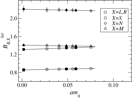
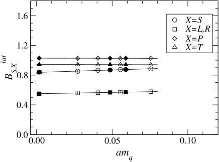
Figure 5: Chiral extrapolation of $B_{B,X}^{lat}$ (top panel) and $B_{S,X}^{lat}$ (bottom panel) at $\beta$ = 6.0 and $aM_{0}$ = 2.1. Data are normalized by their vacuum saturation approximation (VSA). It is $B_{B,L}^{\mathrm{(VSA)}}=1$, $B_{B,S}^{\mathrm{(VSA)}}=-5/8$, $B_{B,N}^{\mathrm{(VSA)}}=1$, $B_{B,M}^{\mathrm{(VSA)}}=-6$ for $B_{B,X}^{lat}$, and $B_{S,S}^{\mathrm{(VSA)}}=1$, $B_{S,L}^{\mathrm{(VSA)}}=-8/5$, $B_{S,P}^{\mathrm{(VSA)}}=-64/5$, $B_{S,T}^{\mathrm{(VSA)}}=288/5$ for $B_{S,X}^{lat}$. In VSA the correction of order $1/M$ is neglected.

The results of $B_{B,X}^{lat}$ and $B_{S,X}^{lat}$ are insensitive to the light quark mass. An example is shown in Figure 5, where the data at $\beta$ = 6.0 are plotted as a function of $am_{q}\equiv\frac{1}{2}\left(\frac{1}{\kappa}-\frac{1}{\kappa_{c}}\right)$. The $B$ parameters for all relevant operators are plotted: $X$ = $L$, $R$, $S$, $N$ and $M$ for $B_{B,X}^{lat}$, and $X$ = $S$, $L$, $R$, $P$, $T$ for $B_{S,X}^{lat}$. Each $B$ parameter is normalized by its vacuum saturation approximation. We averaged the matrix elements with $X$ = $L$ and $R$, as they should be equal in the infinite number of statistics by parity symmetry. In later sections, the averaged matrix elements are denoted by $X$ = $LR$.

We extrapolate these $B$ parameters to the chiral limit of light quark assuming a linear function in $am_{q}$. In most cases the chiral extrapolation changes the value of $B$ parameters from the lightest measured data by about 1% or less. Therefore, the chiral extrapolation is extremely stable and the associated systematic error is negligible. To confirm this observation we also tried a quadratic extrapolation for some parameter sets, for which we find that the results are consistent with the linear extrapolation within the statistical error.

In chiral perturbation theory for heavy-light mesons, the logarithmic dependence such as $m_{q}\ln m_{q}$ is predicted for $B_{B}$ Booth:1995hx ; Sharpe:1996qp . In the quenched approximation the chiral limit is even divergent as $\ln m_{q}$. The more divergent term $\ln m_{q}$ has a factor $1-3g^{2}$ as its coefficient, and the $B^{*}B\pi$ coupling $g$ is evaluated in the range 0.2–0.7 using $D^{*}\rightarrow D\pi$ decay Stewart:1998ke , $D^{*}$ decay width Anastassov:2002cw , quark models Casalbuoni:1997pg , and quenched lattice calculations deDivitiis:1998kj ; Aoki:2001rd ; Abada:2002xe . It means that this divergent logarithm is relatively unimportant because of its small coefficient $1-3g^{2}$ = 0.2(7). It is, however, difficult to resolve such logarithmic dependences from the data taken in the range of our light quark masses. In this work, therefore, we do not further consider them, leaving the study of the chiral logarithm including the effect of unquenching for future publications.

Results of the linear extrapolation are summarized in Table 2–9, where we list the values of $B_{B,X}^{lat}$ and $B_{S,X}^{lat}$ at each $\beta$ and $aM_{0}$. The value of $\kappa$ corresponding to the physical $u$ or $d$ quark mass, which we denote $\kappa_{ud}$, is very close to the critical value $\kappa_{c}$. The value of $\kappa_{s}$ corresponding to the strange quark mass depends on the input quantity. We list the results at $\kappa_{s1}$, for which the $K$ meson mass is used as input, and at $\kappa_{s2}$, for which $\phi$ meson mass is used.

V.3 $1/M_{P}$ dependence

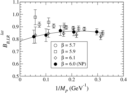
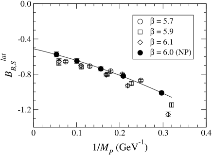
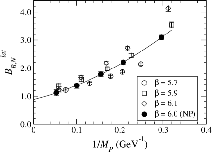
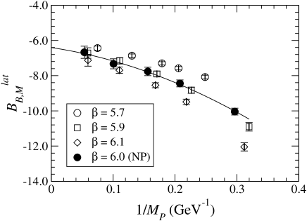
Figure 6: $1/M_{P}$ dependence of the lattice $B$ parameters $B_{B,X}$ ($X$ = $LR$, $S$, $N$ and $M$). A quadratic fit is plotted for the data at $\beta$ = 6.0.

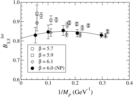
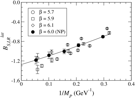
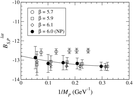
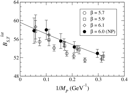
Figure 7: $1/M_{P}$ dependence of the lattice $B$ parameters $B_{S,X}$ ($X$ = $S$, $LR$, $P$ and $T$). A quadratic fit is plotted for the data at $\beta$ = 6.0.

The $1/M_{P}$ dependence of the lattice $B$ parameters $B_{B,X}^{lat}$ ($B_{S,X}^{lat}$) is plotted in Figure 6 (Figure 7). The light quark is extrapolated to the chiral limit. Although the data at different $\beta$ values are overlaid, they do not necessarily agree because the operators are not renormalized. Comparison with an adequate definition (the $B$ parameter in the continuum renormalization scheme) will be discussed in detail in Section V.6.

We find that the mass dependence is small for $B_{B,LR}^{lat}$, while it is significant for others. This behavior can be mostly understood using the vacuum saturation approximation (VSA) Hashimoto:1999ck . In VSA the matrix element in the numerator of the $B$ parameter is generally decomposed into $|\langle 0|A_{\mu}|P\rangle|^{2}$ and $|\langle 0|P|P\rangle|^{2}$. For $B_{B,LR}^{lat}$, however, it is written by $|\langle 0|A_{\mu}|P\rangle|^{2}$ only and no $|\langle 0|P|P\rangle|^{2}$ term appears by definition, so that $B_{B,LR}^{\mathrm{(VSA)}}$ = 1 is independent of $1/M_{P}$. For others, the term $|\langle 0|P|P\rangle|^{2}$ gives a strong mass dependence proportional to $(M_{P}/M)^{2}=(1+\bar{\Lambda}/M)^{2}$, where $\bar{\Lambda}$ represents the binding energy produced by the light degrees of freedom. Comparison of the lattice data with VSA is made in Ref.  Hashimoto:1999ck .

V.4 Renormalized $B$ parameters

The $B$ parameters for the continuum operators are obtained from the lattice $B$ parameters using (49) for $B_{B}$ and (50) for $B_{S}$. We consider the truncation method I in this subsection. The results of other truncations are discussed in the next subsection.

In order to see the effect of $1/M$ corrections we consider the quantity

$$\Phi_{B_{B}}(\mu_{b})\equiv\left(\frac{\alpha_{s}(M_{P})}{\alpha_{s}(M_{B})}\right)^{2/\beta_{0}}B_{B}(\mu_{b})$$ (66)

as a function of $1/M_{P}$. The factor $(\alpha_{s}(M_{P})/\alpha_{s}(M_{B}))^{2/\beta_{0}}$ is introduced to cancel the logarithmic dependence on $M$ coming from the continuum one-loop integral, so that the heavy quark expansion in $1/M_{P}$ is explicit. Up to two-loop corrections $\Phi_{B_{B}}(\mu_{b})$ is equivalent to $B_{B}(\mu_{b})$ obtained with a replacement of $M$ in $\rho_{L,L}$ (43) and in $\rho_{A}^{(0)}$ (28) by the physical $b$ quark mass $m_{b}$, which can be confirmed by expanding the factor $(\alpha_{s}(M_{P})/\alpha_{s}(M_{B}))^{2/\beta_{0}}$ in $\alpha_{s}(M_{P})$ explicitly. With the replacement the static limit ($1/M_{P}\rightarrow 0$) of NRQCD simply becomes the conventional static approximation. Therefore, in the calculation of $\Phi_{B_{B}}(\mu_{b})$ we explicitly set the physical $b$ quark mass $m_{b}$ in the matching coefficients (43) and (28). It should be also noted that at the physical $B$ meson mass, namely $M_{P}$=$M_{B}$, our definition of $\Phi_{B_{B}}(\mu_{b})$ exactly agrees with the definition (66).

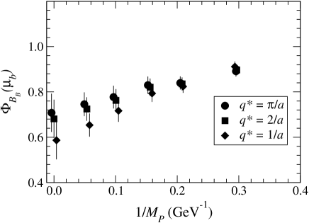
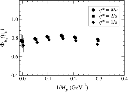
Figure 8: $\Phi_{B_{B}}(\mu_{b})$ (top panel) and $\Phi_{B_{S}}(\mu_{b})$ (bottom panel) for $\mu_{b}=m_{b}$. Data show the result at $\beta=6.0$ in the chiral limit of the light quark. The truncation method I is chosen as a demonstration. Different symbols correspond to different scales of the coupling constant in the perturbative matching, and data points are slightly shifted in the x-direction for clarity. The data at the static limit ($1/M_{P}=0$) is obtained by an extrapolation in $1/M_{P}$ with a quadratic function.

Figure 8 (top panel) shows $\Phi_{B_{B}}(\mu_{b})$ at $\beta=6.0$. The light quark mass is extrapolated to the chiral limit, and the renormalization scale $\mu_{b}$ is set to $m_{b}$. In the one-loop matching (49) we use the renormalized coupling $\alpha_{V}(q^{*})$ defined through the heavy quark potential Lepage:1993xa . The scale $q^{*}$ represents the momentum region where the relevant one-loop integral dominates. Since it is not known, we use three typical values $\pi/a$, $2/a$ and $1/a$ and consider their variation as an indication of systematic uncertainty from higher order perturbative corrections. We find that the variation among different coupling constants becomes substantial as one goes to the static limit, while it is relatively unimportant in the physical mass region $1/M_{P}\sim$ 0.2 GeV^-1. This is because the one-loop coefficients in the matching (49) grows toward the static limit. For the $1/M_{P}$ dependence of $\Phi_{B_{B}}(\mu_{b})$ we observe a slight positive slope and curvature, but the large systematic uncertainty implies that the mass dependence is insignificant.

We obtain a similar plot for $\Phi_{B_{S}}(\mu_{b})$ in Figure 8 (bottom panel), which is an analog of $\Phi_{B_{B}}(\mu_{b})$ but for $B_{S}(\mu_{b})$. The definition of $\Phi_{B_{S}}(\mu_{b})$ with the renormalization group improvement as in (66) is more complicated, since the logarithmic dependence appears in more than one coefficients, so that we have to consider a mixing of operators. In this work, however, we avoid this problem by replacing the heavy quark mass in $\rho_{S,S}$ and $\rho_{S,L}$ by the physical value as we did for $\Phi_{B_{B}}(\mu_{b})$.

For $B_{S}(\mu_{b})$ the one-loop coefficients are relatively small and their dependence on the heavy quark mass is mild. Hence, we obtain a smaller variation due to different scale settings in the coupling constant.

V.5 Effect of truncation of expansions

As we discussed in Section III.4 there are several method to truncate the perturbative and $1/M$ expansions. We consider the following four methods. In the methods I and I’ the perturbative matching is truncated in the numerator and denominator separately as in (49) and (50), while in the methods II and II’ the denominator is linearized as (53) and (54). In the primed methods the heavy quark field without the FWT rotation (22) is used for one-loop correction terms.

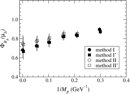
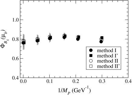
Figure 9: $\Phi_{B_{B}}(\mu_{b})$ (top panel) and $\Phi_{B_{S}}(\mu_{b})$ (bottom panel) for $\mu_{b}=m_{b}$. Data show the result at $\beta=6.0$ in the chiral limit for the light quark and renormalized with the coupling $\alpha_{V}(2/a)$. Different symbols correspond to different truncations of perturbative and heavy quark expansions. The data at the static limit ($1/M_{P}=0$) is obtained by an extrapolation in $1/M_{P}$ with a quadratic function.

In Figure 9 we plot $\Phi_{B_{B}}(\mu_{b})$ (top panel) and $\Phi_{B_{S}}(\mu_{b})$ (bottom panel) for four different truncation methods. As can be seen from the figure, the methods I and I’ (or II and II’) agree in the static limit, since their difference is only in the FWT rotation. On the other hand, the difference between the methods I and II (or I’ and II’) is smaller for lighter heavy quarks because the one-loop correction in the denominator $\rho_{A}^{(0)}$ becomes small.

We consider the variation among different truncations as an indication of systematic uncertainties from higher orders of perturbative and $1/M$ expansions. The error estimation is given in the next section.

V.6 Results at different lattice spacings

Since NRQCD is formulated by an expansion in $1/M$ and not a renormalizable field theory, it does not allow a continuum limit; instead it has to be considered as an effective theory valid in the region where $1/(aM_{0})$ is small enough. The dependence of systematic errors on the lattice spacing $a$ is not just a simple power series in $a$, but contains its inverse powers. Therefore, the question is how one can find a region of $a$ where the discretization error is small while the errors scaling as $1/a^{n}$ ($n$ is a positive integer) is under control. Although the order counting argument as discussed in Hashimoto:1999ck ; Hashimoto:2000eh provides a rough estimate of errors, it is essential to confirm it using actual simulation data.

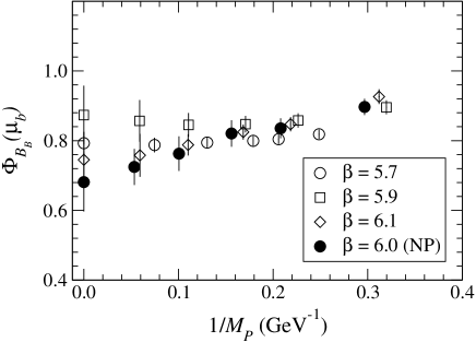
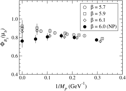
Figure 10: $\Phi_{B_{B}}(\mu_{b})$ (top panel) and $\Phi_{B_{S}}(\mu_{b})$ (bottom panel) for $\mu_{b}=m_{b}$. Results at different lattice spacings are compared. Data show the results in the chiral limit for the light quark and renormalized with the coupling $\alpha_{V}(2/a)$. The truncation method I is chosen as a demonstration. The data at the static limit ($1/M_{P}=0$) is obtained by an extrapolation in $1/M_{P}$ with a quadratic function.

In Figure 10 we plot $\Phi_{B_{B}}(\mu_{b})$ (top panel) and $\Phi_{B_{S}}(\mu_{b})$ (bottom panel) obtained with the truncation method I for four different lattice spacings. The largest (smallest) inverse lattice spacing is 2.3 GeV at $\beta=6.1$ (1.1 GeV at $\beta=5.7$). We find that around the physical $B$ meson mass ($1/M_{B}\sim$ 0.2 GeV^-1) the results agree within order 10% for $\Phi_{B_{B}}(\mu_{b})$ or even better for $\Phi_{B_{S}}(\mu_{b})$. The agreement becomes marginal toward the static limit especially for the nonperturbatively improved lattice ($\beta=6.0$), but it is not statistically significant.

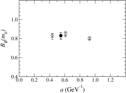
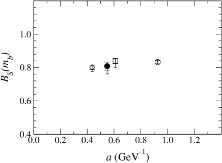
Figure 11: Dependence of $B_{B}(m_{b})$ (top panel) and $B_{S}(m_{b})$ (bottom panel) on the lattice spacing $a$. Data show the results in the chiral limit for the light quark and renormalized with the coupling $\alpha_{V}(2/a)$. The truncation method I is chosen as a demonstration. The variation due to the different choice of fit range is added to the error bar at each $\beta$.

Results of physical $B_{B}(m_{b})$ (top panel) and $B_{S}(m_{b})$ (bottom panel) are plotted in Fig. 11 as a function of the lattice spacing, where the variation due to the different choice of fit range is added to the error bar at each $\beta$. The $a$ dependence is a mixture of the discretization error scaling as $a^{m}$ and the truncation error containing a form like $1/a^{n}$. In addition, the truncation of perturbative expansion gives a functional dependence like $1/\ln a$. It is, therefore, difficult to determine the shape of the $a$ dependence, but the data imply that none of these errors is diverging in the region we measured.

VI Physics results

VI.1 Analysis of systematic errors

As discussed in the previous section, we have performed the calculation of the $B$ parameters with four different truncations of $1/M$ and $\alpha_{s}$ expansions. Furthermore, the calculations are made at four different lattice spacings. All of these calculations have different amount of various systematic errors, and thus they allow us to estimate the uncertainty in our final results. In this subsection we first list possible sources of systematic errors and estimate their size using a naive order counting. Then, their results are compared with the actual lattice data.

One of the possible systematic errors arises from the discretization of derivatives, which scales as a power of the lattice spacing $a$. Because our actions and operators are $O(a)$-improved at tree level, the leading error is of order $a^{2}$ and of order $\alpha_{s}a$. Since we are using an effective theory for heavy quark, the truncation of the $1/M$ expansion leads to a systematic error. For our choice of actions and operators the leading contribution is of order $1/M_{b}^{2}$. Again, since the matching of the $1/M$ terms is done at the tree level only, we also expect an error of order $\alpha_{s}/M_{b}$. The perturbative matching of operators are truncated at the one-loop level, so that there is an uncertainty of order $\alpha_{s}^{2}$. In Table 10 we list their typical size at each $\beta$ value using a naive order counting. Where the scale is needed we assume the typical spatial momentum inside a heavy-light meson to be $p\sim\Lambda_{\mathrm{QCD}}\sim$ 300 MeV. For the strong coupling constant we use a typical value $\alpha_{V}(2/a)$ as listed in Table 1.

The contribution of order $p^{2}/M_{b}^{2}$ is not investigated in this paper, as we just neglect the $1/M^{2}$ terms in the action and operators. In Table 10 we assign 2% as the corresponding uncertainty rather than a naive order counting 0.4%, taking the estimate from explicit lattice study in Hashimoto:1999ck .

Since we have removed errors of $\alpha_{s}/(aM)^{m}$ ($m\geq$0) by perturbative matching, the leading contribution which prevents us from the continuum extrapolation with the NRQCD action has the form $\alpha_{s}^{2}/(aM)$. Although its size in the naive order counting is smaller than the pure two-loop correction $\alpha_{s}^{2}$, we include it in our error analysis (thus in Table 10), as it gives the leading contribution growing toward the continuum limit.

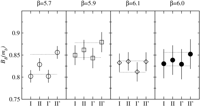
Figure 12: Results for $B_{B}$ at each $\beta$ with four different truncation methods (see text). Comparison is made with the estimate using the naive order counting (a band given by the dotted lines).

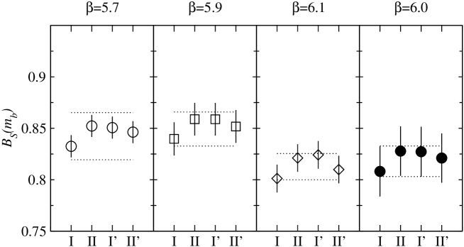
Figure 13: Same as Figure 12, but for $B_{S}$.

As mentioned in Section III.4, the results from the different truncation methods (I, II, I’ and II’) are expected to differ from each other by $O(\alpha_{s}^{2})$ or $O(\alpha_{s}p/M_{b})$. We compare their results in Figure 12 for $B_{B}$ and in Figure 13 for $B_{S}$. The results of the four truncation methods when $\alpha_{s}(2/a)$ is used in the one-loop matching are plotted. In these Figures we also show the size of the systematic errors of order $O(\alpha_{s}^{2})$ and $O(\alpha_{s}p/M_{b})$ estimated with the naive order counting (first two lines of Table 10 added in quadrature). Although the statistical error of the data points makes the comparison somewhat ambiguous, we conclude that the naive order counting reasonably explains the scatter of the lattice data. The same conclusion is reached when we use different values of $q^{*}$ in the perturbative matching.

An alternative way to estimate the $O(\alpha_{s}^{2})$ error is to see the variation of results with $q^{*}$=$\pi/a$, $2/a$ and $1/a$. From Figure 8, where the data at $\beta$ = 6.0 are plotted, we find that the variation with the choice of scale in the coupling constant is consistent with our order counting ($\sim$ 3%) for the data points around the $B$ meson mass. In the static limit, on the other hand, the one-loop coefficient is uncomfortably large, and the variation among the results with different $q^{*}$ is much larger than our naive estimate.

Other sources of systematic errors to be tested are $O(a^{2}p^{2})$, $O(ap\alpha_{s})$ and $O(\alpha_{s}^{2}/(aM_{b}))$. Although it is difficult to disentangle various $a$ dependent systematic errors solely from the data, our results are stable against the change of lattice spacing suggesting that the systematic error is well estimated by the naive order counting.

Finally we also investigated the systematic error from the contamination of excited states by changing the fit range for the ratio $R_{B,X}(t_{1},t_{2})$ and $R_{S,X}(t_{1},t_{2})$. We find that the effect is at most 3%. In particular, at $\beta$=6.0 it is found to be 1% for $B_{B}$ and 3% for $B_{S}$. These variations are taken into account in the final results.

VI.2 $B$ parameter results

As we discussed above, the systematic errors estimated with the naive order counting actually describe the differences among different calculations. We, therefore, use the order counting argument to quote our estimate of systematic uncertainties.

We take the central values from the data at $\beta$ = 6.0 (set $B$) with $q^{*}$=$2/a$, and obtain the following results in the quenched approximation.

$$B_{B}(m_{b}) = 0.84(3)(5),$$ (67)

$$B_{B_{s}}(m_{b}) = 0.86(2)(5)(0),$$ (68)

$$B_{S}(m_{b}) = 0.82(2)(5),$$ (69)

$$B_{S_{s}}(m_{b}) = 0.85(1)(5)(^{+1}_{-0}),$$ (70)

where the first and second errors represent statistical and systematic ones respectively. In the systematic error the contamination from excited states is added in quadrature with other sources estimated by the order counting. The third error is from the uncertainty of $m_{s}$ arising from the different input physical quantities, i.e. $m_{K}$ or $m_{\phi}$.

The corresponding renormalization scale independent $B$ parameter is obtained from (7)

$$\hat{B}_{B}=1.29(5)(8),$$ (71)

which may be compared with the previous calculations using the relativistic actions for heavy quark, 1.38(11)$(^{+0}_{-9})$ Becirevic:2001nv and 1.40(5)$(^{+6}_{-1})$ Lellouch:2001tw . These two results are slightly higher than our result, although Becirevic:2001nv is still consistent within the large error. A possible reason for the high values in the relativistic approach is in the extrapolation in the heavy quark mass from the charm quark mass region to the bottom. In fact, the combined analysis of the HQET and relativistic heavy quark, in which the interpolation in $1/M$ can be made, gives 1.34(6)$(^{+8}_{-6})$ Becirevic:2001xt , i.e. closer to our result.

VI.3 Applications

In this subsection we present a few examples of physics applications of our results. It should be noted, however, that our calculation is still in the quenched approximation and there is no rigorous estimate for the associated uncertainty. For the following applications we assume that the quenching effect is negligible for the $B$ parameters as suggested by our preliminary calculations Hashimoto:2001zq ; Yamada:2001ik ; Yamada:2001xp .

For the $B$ meson decay constant, on the other hand, the large effect of quenching has been found Ryan:2001ej ; Kronfeld:2001ss ; Yamada:2002_rev . Furthermore, a large uncertainty due to the presence of chiral logarithm is suggested for $f_{B}$ Yamada:2002_rev ; Kronfeld:2002ab , while the effect is not too large for $f_{B_{s}}$. In the following analysis we therefore consider the quantities for which only $f_{B_{s}}$ is needed, and use the recent world average of unquenched lattice calculations of $f_{B_{s}}$ = 230(30) MeV Ryan:2001ej ; Yamada:2002_rev when needed.

Assuming the three generation unitarity $|V_{ts}|\simeq|V_{cb}|$, we obtain the mass difference in $B_{s}^{0}-\bar{B}_{s}^{0}$ mixing using (2) as

$$\Delta M_{s}=19.4(5.5)~{}\mbox{ps}^{-1},$$ (72)

where the statistical and systematic errors in theoretical and experimental quantities are added in quadrature, but the final error is dominated by the uncertainty of $f_{B_{s}}$. The value is consistent with the current lower bound $\Delta M_{s}>13.1$ ps^-1 at a 95% CL PDG2002 . Tevatron Run II is expected to measure the mass difference very precisely in a few years.

The width difference in the $B_{s}$ meson system could also be measured at Tevatron Run II, if it is large enough. Using (15) and (70), we obtain

$$\left(\frac{\Delta\Gamma}{\Gamma}\right)_{B_{s}}=0.106\pm 0.020\pm 0.028\pm 0.037\pm 0.024,$$ (73)

where the first through third errors are from $m_{b}$ = 4.8(3) GeV, $f_{B_{s}}$ = 230(30) MeV, and $\mathcal{R}$ (or $\bar{m}_{b}(m_{b})$ = 4.25(25) GeV and $\bar{m}_{s}(m_{b})$ = 0.10(3) GeV), respectively. The last error comes from the uncertainty in the estimation of the $1/m$ correction, for which we assign 30%. The error from the $B$ parameters is much smaller than the others listed above.

The uncertainty in the calculation of $(\Delta\Gamma/\Gamma)_{B_{s}}$ is still very large ($\sim$ 50% if added in quadrature). In order to improve it one has to calculate the $1/m$ corrections reliably, as it largely cancels the leading contribution from $B_{S}$ as seen in (15). Currently, only an upper bound is obtained for this quantity experimentally. Our prediction is consistent with the bound $(\frac{\Delta\Gamma}{\Gamma})_{B_{s}}<0.31$ at a 95 % CL PDG2002 .

VII SU(3) breaking ratio $\xi$

Since we expect that the bulk of systematic uncertainty in the calculation of $f_{B}$ and $B_{B}$ cancels in their SU(3) breaking ratio $f_{B_{s}}/f_{B}$ and $B_{B_{s}}/B_{B}$, they could be useful to reduce the errors in the determination of $|V_{td}|$ through the relation (8).

In the lattice calculation, the deviation of their ratio from unity is the quantity to be calculated and the errors scale as $B_{B_{s}}/B_{B}-1$ rather than $B_{B_{s}}/B_{B}$ itself. In the present case, the naive estimate of SU(3) breaking is $O(m_{K}^{2}/\Lambda_{\chi}^{2})\sim$ 25%, where $\Lambda_{\chi}$ is a scale of the chiral symmetry breaking $\sim$ 1 GeV, and the order counting of uncertainties for the ratio are starting from this order.

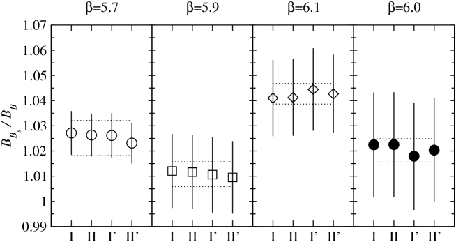
Figure 14: Same as Figure 12, but for $B_{B_{s}}/B_{B}$.

As done in Section VI.1, we compare our order counting with data in Figure 14. As we expected, the variation with different truncations is much smaller than the expected systematic errors (dotted line). The dependence on $\beta$ is sizable, but not significant compared to the relatively large statistical error.

Our result is

$$\frac{B_{B_{s}}}{B_{B}}=1.020(21)(^{+15}_{-16})(^{+5}_{-0}),$$ (74)

where the central value is taken from $\beta$ = 6.0 (set B), and the errors are statistical, systematic and the uncertainty of $m_{s}$ in the order given.

For the calculation of $\xi$ (1) we have to combine $B_{B_{s}}/B_{B}$ with $f_{B_{s}}/f_{B}$, which is called the indirect method. On the other hand, it is also possible to directly obtain $\xi$ from a ratio of $\langle O_{L_{s}}\rangle$ and $\langle O_{L_{d}}\rangle$ (direct method). It has been discussed that one may obtain rather large value of $\xi$ if one uses the direct method Bernard:1998dg ; Lellouch:2001tw . Therefore, in the following we check if we could obtain consistent results from both methods using our data.

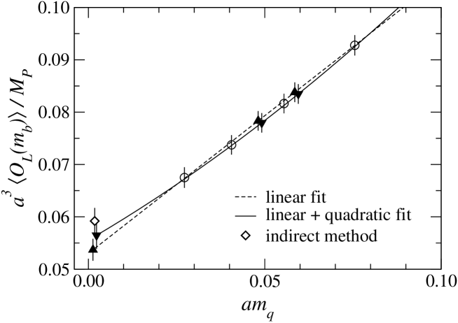
Figure 15: Comparison of direct and indirect methods. The dashed line is a linear fit and the solid curve is obtained with a fit with linear and quadratic terms. An open diamond at the chiral limit is obtained through the indirect method.

Figure 15 shows the chiral extrapolation of $\langle O_{L}\rangle$, as required in the direct method. The data are obtained at $\beta$ = 6.0 (set B) for a heavy quark mass closest to the $b$ quark mass. The dashed line is obtained by a linear fit to the data (open circles), while the solid curve represents a fit with a linear plus quadratic term in $am_{q}$. Although the data look consistent with the linear fit, the chiral limit with the quadratic fit is higher by about one standard deviation.

An open diamond at the chiral limit, on the other hand, is obtained through the indirect method, i.e. the decay constant and $B$ parameter are separately extrapolated to the chiral limit with a linear fit. Although we have not presented a calculation of the decay constant in this paper, they are done on the same set of gauge configurations at $\beta$ = 6.0 and the lattice axial current is renormalized as described in Section III.2. The result is completely consistent with the quadratic fit in the direct method. It implies that in the direct method the chiral extrapolation is more difficult and needs enough statistics to control, since $\langle O_{L}\rangle$ is effectively the decay constant squared so that the finite $am_{q}$ correction is amplified.

VIII Conclusions

In this work, we calculate the $B$ meson $B$ parameters on the lattice in the quenched approximation. The calculation is an extension of our previous works Hashimoto:1999ck ; Hashimoto:2000yh , in which $B_{B}$ and $B_{S}$ were calculated for the first time with the lattice NRQCD action.

In the present work we include a detailed study of systematic uncertainties. Using the lattice simulations at four different $\beta$ values with the $O(a)$-improved actions, we find that the $B$ parameters are essentially insensitive to the discretization error. We also investigate the systematic errors associated with the truncation of heavy quark and perturbative expansions, which are necessary in the effective theory approach such as NRQCD. By comparing four different truncations of these expansions, we are able to confirm that the naive order counting argument of the systematic errors could actually give a reasonable estimate.

In our final results for the $B$ parameters the systematic error is $\sim$ 6%, which is already smaller than that in the equivalent calculations of $f_{B}$ (10–20%), owing to the fact that it is defined as a ratio to the vacuum saturation approximation. Further reduction of systematic errors, if it is necessary, requires higher order calculation of perturbation theory and the $O(a^{2})$ improvement. Approaching to the continuum limit will not help to reduce the errors in the NRQCD approach.

For a precise extraction of the important CKM element $|V_{td}|$ through the SU(3) breaking ratio of the $B-\bar{B}$ mixing one needs $\xi^{2}$. It is preferable to take the chiral limit separately for $f_{B}$ and $B_{B}$, as they have milder light quark mass dependence. The SU(3) breaking ratio of $B_{B}$ is obtained with accuracy of order a few percent, since the $B$ parameter is extremely insensitive to the light quark mass and the large cancellation of systematic errors is expected.

The largest remaining uncertainty in our calculation is in the quenching approximation, though it is not explicitly discussed in the paper. We are currently performing an unquenched simulation with the same lattice action at similar lattice spacing, which will allow us to directly study the quenching effect.

set	A			B
$\beta$	6.1	5.9	5.7	6.0
size	$24^{3}\times 64$	$16^{3}\times 48$	$12^{3}\times 32$	$20^{3}\times 48$
#conf	518	419	420	655
$c_{\mathrm{SW}}$	1.525	1.580	1.674	1.769
$1/a$ (GeV)	2.29	1.64	1.08	1.82
$\kappa$	0.13586	0.13630	0.13690	0.13260
	0.13642	0.13711	0.13760	0.13331
	0.13684	0.13769	0.13840	0.13384
	0.13716	0.13816	0.13920	0.13432
$\kappa_{s1}$	0.13635	0.13702	0.13800	0.13355
$\kappa_{s2}$	0.13609	0.13657	0.13707	0.13318
$\kappa_{c}$	0.13767	0.13901	0.14157	0.13531
$(aM_{0},n)$	(7.0,2)	(10.0,2)	(12.0,2)	(10.0,2)
	(3.5,2)	(5.0,2)	(6.5,2)	(5.0,2)
	(2.1,2)	(3.0,2)	(4.5,2)	(3.0,2)
	(1.5,3)	(2.1,3)	(3.8,2)	(2.1,3)
	(0.9,4)	(1.3,3)	(3.0,2)	(1.3,3)
$[t_{1min},t_{1max}]$	[8,26]	[6,17]	[4,13]	[ 7,18] for $aM_{0}$ = 10.0
				[ 9,18] for $aM_{0}$ = 5.0
				[10,18] for $aM_{0}$ = 3.0, 2.1, 1.3
$u_{0}$	0.8816	0.8734	0.86087	0.87603
$\alpha_{V}(\pi/a)$	0.149	0.164	0.188	0.159
$\alpha_{V}(2/a)$	0.172	0.193	0.229	0.186
$\alpha_{V}(1/a)$	0.229	0.270	0.355	0.256

Table 1: Simulation parameters. For the simulation set A, the $O(a)$-improvement coefficient $c_{\mathrm{SW}}$ is determined at the tadpole-improved one-loop level. For the set B, the nonperturbatively tuned value Luscher:1997ug is used.

$aM_{0}$	12.0	6.5	4.5	3.8	3.0
$B^{lat}_{B,LR}$
$\kappa_{ud}$	0.916(21)	0.906(17)	0.894(15)	0.889(14)	0.882(14)
$\kappa_{s1}$	0.931(13)	0.923(11)	0.915(09)	0.911(09)	0.905(09)
$\kappa_{s2}$	0.934(12)	0.927(09)	0.920(08)	0.916(08)	0.911(08)
$B^{lat}_{B,S}$
$\kappa_{ud}$	$-$0.656(11)	$-$0.708(10)	$-$0.765(10)	$-$0.802(11)	$-$0.870(12)
$\kappa_{s1}$	$-$0.659(07)	$-$0.713(06)	$-$0.770(07)	$-$0.806(07)	$-$0.872(08)
$\kappa_{s2}$	$-$0.659(06)	$-$0.714(06)	$-$0.772(06)	$-$0.808(06)	$-$0.872(08)
$B^{lat}_{B,N}$
$\kappa_{ud}$	1.220(36)	1.459(31)	1.707(32)	1.864(34)	2.144(40)
$\kappa_{s1}$	1.212(23)	1.444(20)	1.683(21)	1.831(23)	2.095(27)
$\kappa_{s2}$	1.210(20)	1.440(17)	1.676(19)	1.822(20)	2.081(24)
$B^{lat}_{B,M}$
$\kappa_{ud}$	$-$6.44(11)	$-$6.87(10)	$-$7.30(09)	$-$7.58(10)	$-$8.08(10)
$\kappa_{s1}$	$-$6.44(07)	$-$6.87(06)	$-$7.31(06)	$-$7.58(07)	$-$8.06(07)
$\kappa_{s2}$	$-$6.44(07)	$-$6.87(06)	$-$7.31(06)	$-$7.58(06)	$-$8.06(07)

Table 2: Numerical values for lattice $B$ parameters $B^{lat}_{B,X}$ at $\beta$=5.7.

$aM_{0}$	12.0	6.5	4.5	3.8	3.0
$B^{lat}_{S,S}$
$\kappa_{ud}$	0.931(15)	0.909(11)	0.894(10)	0.887(10)	0.879(09)
$\kappa_{s1}$	0.941(10)	0.927(07)	0.916(07)	0.910(06)	0.904(06)
$\kappa_{s2}$	0.944(09)	0.931(07)	0.922(06)	0.917(06)	0.910(05)
$B^{lat}_{S,LR}$
$\kappa_{ud}$	$-$1.301(31)	$-$1.163(23)	$-$1.044(19)	$-$0.982(18)	$-$0.891(17)
$\kappa_{s1}$	$-$1.330(19)	$-$1.200(14)	$-$1.088(12)	$-$1.028(12)	$-$0.938(11)
$\kappa_{s2}$	$-$1.338(17)	$-$1.209(13)	$-$1.099(11)	$-$1.040(10)	$-$0.951(10)
$B^{lat}_{S,P}$
$\kappa_{ud}$	$-$12.59(18)	$-$12.56(15)	$-$12.52(14)	$-$12.51(13)	$-$12.51(12)
$\kappa_{s1}$	$-$12.66(12)	$-$12.68(10)	$-$12.69(09)	$-$12.69(09)	$-$12.70(08)
$\kappa_{s2}$	$-$12.68(10)	$-$12.71(09)	$-$12.73(08)	$-$12.74(08)	$-$12.76(08)
$B^{lat}_{S,T}$
$\kappa_{ud}$	55.43(87)	54.09(67)	52.91(58)	52.31(55)	51.45(50)
$\kappa_{s1}$	55.79(57)	54.72(45)	53.77(39)	53.27(37)	52.50(35)
$\kappa_{s2}$	55.89(51)	54.90(40)	54.01(36)	53.53(34)	52.78(32)

Table 3: Numerical values for lattice $B$ parameters $B^{lat}_{S,X}$ at $\beta$=5.7.

$aM_{0}$	10.0	5.0	3.0	2.1	1.3
$B^{lat}_{B,LR}$
$\kappa_{ud}$	0.977(61)	0.936(35)	0.904(25)	0.884(22)	0.848(22)
$\kappa_{s1}$	0.956(34)	0.931(19)	0.911(13)	0.897(12)	0.871(12)
$\kappa_{s2}$	0.952(30)	0.930(16)	0.913(11)	0.899(10)	0.877(11)
$B^{lat}_{B,S}$
$\kappa_{ud}$	$-$0.669(32)	$-$0.718(19)	$-$0.800(16)	$-$0.904(17)	$-$1.148(25)
$\kappa_{s1}$	$-$0.650(17)	$-$0.715(10)	$-$0.805(09)	$-$0.911(10)	$-$1.150(17)
$\kappa_{s2}$	$-$0.646(15)	$-$0.714(09)	$-$0.806(08)	$-$0.912(09)	$-$1.150(15)
$B^{lat}_{B,N}$
$\kappa_{ud}$	1.346(122)	1.595(74)	1.979(60)	2.453(67)	3.541(102)
$\kappa_{s1}$	1.288(070)	1.560(41)	1.935(35)	2.381(41)	3.395(066)
$\kappa_{s2}$	1.275(060)	1.552(35)	1.924(31)	2.364(37)	3.361(059)
$B^{lat}_{B,M}$
$\kappa_{ud}$	$-$6.715(297)	$-$7.156(182)	$-$7.903(162)	$-$8.828(177)	$-$10.904(241)
$\kappa_{s1}$	$-$6.521(176)	$-$7.087(104)	$-$7.862(093)	$-$8.742(102)	$-$10.684(145)
$\kappa_{s2}$	$-$6.476(157)	$-$7.071(091)	$-$7.852(082)	$-$8.723(090)	$-$10.634(128)

Table 4: Numerical values for lattice $B$ parameters $B^{lat}_{B,X}$ at $\beta$=5.9.

$aM_{0}$	10.0	5.0	3.0	2.1	1.3
$B^{lat}_{S,S}$
$\kappa_{ud}$	0.942(44)	0.907(23)	0.882(15)	0.868(13)	0.848(11)
$\kappa_{s1}$	0.923(24)	0.912(12)	0.899(08)	0.888(07)	0.873(06)
$\kappa_{s2}$	0.918(21)	0.913(11)	0.902(07)	0.893(06)	0.878(06)
$B^{lat}_{S,LR}$
$\kappa_{ud}$	$-$1.376(85)	$-$1.184(45)	$-$0.999(30)	$-$0.850(25)	$-$0.627(22)
$\kappa_{s1}$	$-$1.357(48)	$-$1.188(24)	$-$1.018(16)	$-$0.875(15)	$-$0.662(14)
$\kappa_{s2}$	$-$1.353(42)	$-$1.188(21)	$-$1.022(14)	$-$0.880(13)	$-$0.670(12)
$B^{lat}_{S,P}$
$\kappa_{ud}$	$-$13.24(55)	$-$13.08(31)	$-$13.10(24)	$-$13.20(22)	$-$13.33(22)
$\kappa_{s1}$	$-$12.90(31)	$-$13.02(17)	$-$13.10(13)	$-$13.17(12)	$-$13.27(12)
$\kappa_{s2}$	$-$12.82(27)	$-$13.01(15)	$-$13.10(12)	$-$13.17(11)	$-$13.25(10)
$B^{lat}_{S,T}$
$\kappa_{ud}$	57.69(233)	55.84(126)	54.53(96)	53.71(89)	52.33(88)
$\kappa_{s1}$	56.36(138)	55.71(072)	54.75(55)	53.86(50)	52.36(49)
$\kappa_{s2}$	56.05(122)	55.68(063)	54.80(48)	53.90(43)	52.36(42)

Table 5: Numerical values for lattice $B$ parameters $B^{lat}_{S,X}$ at $\beta$=5.9.

$aM_{0}$	7.0	3.5	2.1	1.5	0.9
$B^{lat}_{B,LR}$
$\kappa_{ud}$	0.833(66)	0.846(32)	0.845(23)	0.834(22)	0.819(24)
$\kappa_{s1}$	0.892(37)	0.892(18)	0.882(12)	0.871(12)	0.857(13)
$\kappa_{s2}$	0.904(33)	0.901(16)	0.889(11)	0.878(10)	0.865(12)
$B^{lat}_{B,S}$
$\kappa_{ud}$	$-$0.653(30)	$-$0.701(17)	$-$0.808(14)	$-$0.929(16)	$-$1.255(28)
$\kappa_{s1}$	$-$0.658(18)	$-$0.725(10)	$-$0.836(09)	$-$0.958(11)	$-$1.282(20)
$\kappa_{s2}$	$-$0.659(16)	$-$0.730(09)	$-$0.842(08)	$-$0.964(10)	$-$1.287(19)
$B^{lat}_{B,N}$
$\kappa_{ud}$	1.227(112)	1.674(61)	2.179(55)	2.715(66)	4.130(115)
$\kappa_{s1}$	1.294(064)	1.689(37)	2.181(35)	2.700(44)	4.047(078)
$\kappa_{s2}$	1.307(057)	1.692(34)	2.181(33)	2.697(41)	4.031(073)
$B^{lat}_{B,M}$
$\kappa_{ud}$	$-$7.125(338)	$-$7.690(180)	$-$8.545(143)	$-$9.490(155)	$-$12.046(230)
$\kappa_{s1}$	$-$6.857(220)	$-$7.575(112)	$-$8.452(089)	$-$9.389(099)	$-$11.877(156)
$\kappa_{s2}$	$-$6.804(204)	$-$7.552(102)	$-$8.433(082)	$-$9.369(092)	$-$11.843(146)

Table 6: Numerical values for lattice $B$ parameters $B^{lat}_{B,X}$ at $\beta$=6.1.

$aM_{0}$	7.0	3.5	2.1	1.5	0.9
$B^{lat}_{S,S}$
$\kappa_{ud}$	0.892(40)	0.843(20)	0.834(13)	0.831(12)	0.827(11)
$\kappa_{s1}$	0.907(24)	0.879(11)	0.869(7)	0.863(7)	0.855(7)
$\kappa_{s2}$	0.910(21)	0.886(10)	0.876(7)	0.870(6)	0.861(6)
$B^{lat}_{S,LR}$
$\kappa_{ud}$	$-$1.138(92)	$-$1.016(41)	$-$0.870(26)	$-$0.741(22)	$-$0.536(19)
$\kappa_{s1}$	$-$1.229(52)	$-$1.080(23)	$-$0.916(15)	$-$0.784(13)	$-$0.571(12)
$\kappa_{s2}$	$-$1.247(46)	$-$1.094(21)	$-$0.925(14)	$-$0.792(12)	$-$0.578(12)
$B^{lat}_{S,P}$
$\kappa_{ud}$	$-$13.09(54)	$-$13.27(26)	$-$13.31(19)	$-$13.32(18)	$-$13.35(17)
$\kappa_{s1}$	$-$13.01(35)	$-$13.28(17)	$-$13.31(12)	$-$13.31(11)	$-$13.31(11)
$\kappa_{s2}$	$-$12.99(33)	$-$13.28(15)	$-$13.31(11)	$-$13.31(10)	$-$13.31(10)
$B^{lat}_{S,T}$
$\kappa_{ud}$	58.65(260)	56.91(124)	55.23(85)	53.90(76)	51.70(68)
$\kappa_{s1}$	57.32(171)	56.66(078)	55.11(53)	53.78(47)	51.65(42)
$\kappa_{s2}$	57.06(158)	56.61(072)	55.08(48)	53.76(43)	51.63(38)

Table 7: Numerical values for lattice $B$ parameters $B^{lat}_{S,X}$ at $\beta$=6.1.

$aM_{0}$	10.0	5.0	3.0	2.1	1.3
$B^{lat}_{B,LR}$
$\kappa_{ud}$	0.820(53)	0.832(51)	0.868(39)	0.857(30)	0.858(25)
$\kappa_{s1}$	0.864(37)	0.869(29)	0.888(22)	0.877(17)	0.872(15)
$\kappa_{s2}$	0.874(34)	0.877(25)	0.892(18)	0.881(14)	0.875(13)
$B^{lat}_{B,S}$
$\kappa_{ud}$	$-$0.574(28)	$-$0.649(27)	$-$0.738(23)	$-$0.820(20)	$-$1.011(22)
$\kappa_{s1}$	$-$0.601(21)	$-$0.673(17)	$-$0.757(14)	$-$0.840(12)	$-$1.029(14)
$\kappa_{s2}$	$-$0.607(19)	$-$0.678(15)	$-$0.761(12)	$-$0.845(11)	$-$1.033(13)
$B^{lat}_{B,N}$
$\kappa_{ud}$	1.128(107)	1.376(97)	1.787(84)	2.207(75)	3.095(81)
$\kappa_{s1}$	1.148(073)	1.393(57)	1.785(48)	2.184(45)	3.023(53)
$\kappa_{s2}$	1.152(066)	1.397(49)	1.784(41)	2.178(39)	3.007(48)
$B^{lat}_{B,M}$
$\kappa_{ud}$	$-$6.67(36)	$-$7.33(28)	$-$7.76(24)	$-$8.44(20)	$-$10.04(20)
$\kappa_{s1}$	$-$6.68(24)	$-$7.15(17)	$-$7.69(14)	$-$8.35(12)	$-$ 9.88(13)
$\kappa_{s2}$	$-$6.68(23)	$-$7.11(15)	$-$7.67(12)	$-$8.33(11)	$-$ 9.84(12)

Table 8: Numerical values for lattice $B$ parameters $B^{lat}_{B,X}$ at $\beta$=6.0.

$aM_{0}$	10.0	5.0	3.0	2.1	1.3
$B^{lat}_{S,S}$
$\kappa_{ud}$	0.829(40)	0.847(35)	0.854(26)	0.840(19)	0.830(14)
$\kappa_{s1}$	0.868(30)	0.881(22)	0.881(15)	0.869(11)	0.857(08)
$\kappa_{s2}$	0.877(28)	0.888(20)	0.887(13)	0.875(10)	0.863(07)
$B^{lat}_{S,LR}$
$\kappa_{ud}$	$-$1.184(77)	$-$1.085(68)	$-$1.005(48)	$-$0.879(33)	$-$0.705(23)
$\kappa_{s1}$	$-$1.249(53)	$-$1.138(39)	$-$1.034(27)	$-$0.907(19)	$-$0.726(14)
$\kappa_{s2}$	$-$1.264(50)	$-$1.149(34)	$-$1.040(23)	$-$0.913(16)	$-$0.730(13)
$B^{lat}_{S,P}$
$\kappa_{ud}$	$-$12.87(58)	$-$13.17(47)	$-$13.13(37)	$-$13.17(28)	$-$13.32(22)
$\kappa_{s1}$	$-$12.95(41)	$-$13.02(27)	$-$13.11(22)	$-$13.14(17)	$-$13.26(14)
$\kappa_{s2}$	$-$12.97(38)	$-$12.99(24)	$-$13.11(19)	$-$13.14(15)	$-$13.24(12)
$B^{lat}_{S,T}$
$\kappa_{ud}$	57.82(276)	58.01(211)	55.59(161)	54.30(118)	52.93(88)
$\kappa_{s1}$	57.99(194)	56.99(126)	55.44(094)	54.21(072)	52.78(57)
$\kappa_{s2}$	58.02(180)	56.76(111)	55.41(082)	54.19(063)	52.74(51)

Table 9: Numerical values for lattice $B$ parameters $B^{lat}_{S,X}$ at $\beta$=6.0.

$\beta$	5.7	5.9	6.1	6.0
$O(\alpha_{s}^{2})$	5%	4%	3%	3%
$O(\alpha_{s}p/M_{b})$	1%	1%	1%	1%
$O(a^{2}p^{2})$	8%	3%	2%	3%
$O(ap\alpha_{s})$	6%	4%	2%	3%
$O(\alpha_{s}^{2}/(aM_{b}))$	1%	1%	1%	1%
$O(p^{2}/M_{b}^{2})$	2 %
Total (added in quadrature)	11 %	7%	5 %	6 %

Table 10: Estimate of systematic uncertainties by a naive dimensional counting at each $\beta$ value.

Figure 1: $R_{B,L}(t_{1},t_{2})$ (top) and $R_{S,S}(t_{1},t_{2})$ (middle) at $\beta$ = 5.7, $aM_{0}$ = 3.8 and $\kappa$ = 0.13920. Horizontal line represents a fit with a range $t_{1}=[4,13]$ for a fixed $t_{2}=4$. The bottom plot shows an effective mass for two point functions $C_{A}^{(2)}(t)$ (open symbols) and $C_{A}^{(2)LS}(t)$ (filled symbols). Circles and squares represent data points for positive and negative $t$ respectively.

Figure 2: Same as Fig. 1, but for $\beta$ = 5.9, $aM_{0}$ = 2.1 and $\kappa$ = 0.13816. Horizontal line represents a fit with a range $t_{1}=[6,20]$ for a fixed $t_{2}=6$.

Figure 3: Same as Fig. 1, but for $\beta$ = 6.1, $aM_{0}$ = 1.5 and $\kappa$ = 0.13716. Horizontal line represents a fit with a range $t_{1}=[8,28]$ for a fixed $t_{2}=8$.

Figure 4: Same as Fig. 1, but for $\beta$ = 6.0, $aM_{0}$ = 2.1 and $\kappa$ = 0.13432. Horizontal line represents a fit with a range $t_{1}=[10,18]$ for a fixed $t_{2}=10$.