Computational Methods for UV-Suppressed Fermions

Abstract.

Lattice fermions with suppressed high momentum modes solve the ultraviolet slowing down problem in lattice QCD. This paper describes a stochastic evaluation of the effective action of such fermions. The method is a based on the Lanczos algorithm and it is shown to have the same complexity as in the case of standard fermions.

1. Introduction

There has been recent interest in the so-called ‘Ultraviolet slowing down’ of fermionic simulations in lattice QCD [Irving et al, 1998, Duncan, Eichten and Thacker, 1999, de Forcrand, 1999, Peardon, Lattice2001, A. Hasenfratz & Knechtli, 2001]. These studies try to address algortmically large fluctuations of the high end modes of the fermion determinant. The goal is to increase the signal-to-noise ratio of the infrared modes and to accelerate fermion simulations as well.

In fact, all the computational effort needed to treat UV-modes by above algorithms can be reduced to zero by suppressing them in the first place [Boriçi, 2002]. The lattice Dirac operator of this fermion theory is given by:

(1.1) $$D=\frac{\mu}{a}\Gamma_{5}\tanh\frac{a\Gamma_{5}D_{W/S/O}}{\mu}$$

where $D_{W/s/o}$ is the input lattice Dirac operator, $a$ the lattice spacing and $\mu>0$ is a dimensionless parameter. For Wilson (W) and overlap (o) fermions as the input theory one has $\Gamma_{5}=\gamma_{5}$. For staggered fermions $\Gamma_{5}$ is a diagonal matrix with entries $+1/-1$ on even/odd lattice sites. The theory converges to the input theory in the contimuum limit and is local and unitary as shown in detail in [Boriçi, 2002]. The input theory is also recovered in the limit $\mu\rightarrow\infty$. For $\mu\rightarrow 0$ one has $D\rightarrow\mu$, i.e. a quenched theory.

Perturbative calculations with this theory are straightforward. To fix the idea I assume in the following Wilson fermions to be input fermions. The inverse fermion propagator is given by

(1.2) $${\tilde{D}}(p)=\frac{\mu}{a}\gamma_{5}\tanh\frac{a{\tilde{H}_{W}}(p)}{\mu}$$

with $p=\{p_{\nu},\nu=1,\ldots,4\}$ being the four-momentum vector. As usual, gauge fields are parametrized by $su(3)$ elements:

(1.3) $$U(x)_{\nu}=e^{iagA(x)_{\nu}},~{}~{}~{}~{}A(x)_{\nu}\in su(3)$$

and the Wilson operator is written as a sum of the free and interaction terms:

$$D_{W}=D_{W}^{0}+D_{W}^{I}$$

The splitting of the lattice Dirac operator is written in the same form:

$$D=D^{0}+D^{I},~{}~{}~{}~{}D^{0}=\frac{\mu}{a}\gamma_{5}\tanh\frac{aH_{W}^{0}}{\mu}$$

where the interaction term has to be determined. This can be done by expanding $D$ in terms of $a/\mu$:

(1.4) $$D=D_{W}[\text{1\kern-2.41109ptl}+c_{1}(\frac{aH_{W}}{\mu})^{2}+c_{2}(\frac{aH_{W}}{\mu})^{4}+\cdots]$$

where $c_{1},c_{2},\ldots$ are real expansion coefficients. Calculation of $D^{I}$ is an easy task if one stays with a finite number of terms in the right hand side of (1.4). Also, the number of terms can be minimized using a Chebyshev approximation for the hyperbolic tangent.

In this paper I describe computational methods needed to evaluate the effective action of the theory defined above. In particular, the complexity of the proposed Lanczos method does not depend on the input sparse matrix that describes a fermion theory on the lattice.

In the following section I derive a class of Lanczos based methods for computations with the proposed theory and then in section 3 conclusions follow.

2. Lanczos based methods for computations with fermions

The effective action of the theory defined above can be written as:

(2.1) $$S_{\text{eff}}=\text{tr}f(A)$$

where $A\in\mathbb{C}^{N\times N}$ and $f(s)$ is a real and smooth function of $s\in\mathbb{R}^{+}$. The matrix $A$ is assumed to be Hermitian and positive definite. Since the trace is difficult to obtain one can use the stochastic method of [Bai et al, 1996]. The method is based on evaluations of many bilinear forms of the type:

(2.2) $${\mathcal{F}}(b,A)=b^{T}f(A)b$$

where $b\in\mathbb{R}^{N}$ is a random vector. The trace is estimated as an average over many bilinear forms. A confidence interval can be computed as described in detail in [Bai et al, 1996].

The method described here is similar to the method of [Bai et al, 1996]. Its viability for lattice QCD computations has been demonstrated in the recent work of [Cahill et al, 1999]. [Bai et al, 1996] derive their method using quadrature rules and Lanczos polynomials. Here, I give an alternative derivation which uses familiar tools (in lattice simulations) such as sparse matrix invertions and Padé approximations. The Lanczos method enters the derivation as an algorithm for solving linear systems of the form:

(2.3) $$Ax=b,~{}~{}~{}~{}~{}~{}x\in\mathbb{C}^{N}$$

2.1. Lanczos algorithm

I follow standard standard texts as [Golub & Van Loan, 1989] and notations and arguments of [Boriçi, 1999b, Boriçi, 2000a, Boriçi, 2000b]. $n$ steps of the Lanczos algorithm [Lanczos, 1952] on the pair $(A,b)$ are given by Algorithm 1.

Algorithm 1 The Lanczos algorithm

  Set $\beta_{0}=0,~{}q_{0}=o,~{}q_{1}=b/||b||^{2}$

  for $~{}i=1,\ldots n$ do

     $v=Aq_{i}$

     $\alpha_{i}=q_{i}^{{\dagger}}v$

     $v:=v-q_{i}\alpha_{i}-q_{i-1}\beta_{i-1}$

     $\beta_{i}=||v||_{2}$

     $q_{i+1}=v/\beta_{i}$

  end for

The Lanczos vectors $q_{1},\ldots,q_{n}\in\mathbb{C}^{N}$ can be compactly denoted by the matrix $Q_{n}=[q_{1},\ldots,q_{n}]$. They are a basis of the Krylov subspace $\mathcal{K}_{n}=\text{span}\{b,Ab,\ldots,A^{n-1}b\}$. It can be shown that the following identity holds:

(2.4) $$AQ_{n}=Q_{n}T_{n}+\beta_{n}q_{n+1}e_{n}^{T},~{}~{}~{}~{}~{}q_{1}=b/||b||_{2}$$

$e_{n}$ is the last column of the identity matrix ${\text{1\kern-2.41109ptl}}_{n}\in\mathbb{R}^{n\times n}$ and $T_{n}$ is the tridiagonal and symmetric Lanczos matrix (2.5) given by:

(2.5) $$T_{n}=\begin{pmatrix}\alpha_{1}&\beta_{1}&&\\ \beta_{1}&\alpha_{2}&\ddots&\\ &\ddots&\ddots&\beta_{n-1}\\ &&\beta_{n-1}&\alpha_{n}\\ \end{pmatrix}$$

The matrix (2.5) is usually referred to as the Lanczos matrix. Its eigenvalues, the so called Ritz values, tend to approximate the extreme eigenvalues of the original matrix $A$.

To solve the linear system (2.3) I seek an approximate solution $x_{n}\in\mathcal{K}_{n}$ as a linear combination of the Lanczos vectors:

(2.6) $$x_{n}=Q_{n}y_{n},~{}~{}~{}~{}~{}y_{n}\in\mathbb{C}^{n}$$

and project the linear system (2.3) on to the Krylov subspace $\mathcal{K}_{n}$:

$$Q_{n}^{{\dagger}}AQ_{n}y_{n}=Q_{n}^{{\dagger}}b=Q_{n}^{{\dagger}}q_{1}||b||_{2}$$

Using (2.4) and the orthonormality of Lanczos vectors, I obtain:

$$T_{n}y_{n}=e_{1}||b||_{2}$$

where $e_{1}$ is the first column of the identity matrix ${\text{1\kern-2.41109ptl}}_{n}$. By substituting $y_{n}$ into (2.6) one obtains the approximate solution:

(2.7) $$x_{n}=Q_{n}T_{n}^{-1}e_{1}||b||_{2}$$

2.2. Algorithms for the bilinear form (2.2)

The theoretical framework of the algorithm of [Bai et al, 1996] can be based on the Padé approximant of the smooth and bounded function $f(.)$ in an interval. The Padé approximation can be expressed as a partial fraction expansion. Therefore, one can write:

(2.8) $$f(s)\approx\sum_{k=1}^{m}\frac{c_{k}}{s+d_{k}}$$

with $c_{k}\in\mathbb{R},d_{k}\geq 0,k=1,\ldots,m$. It is assumed that the right hand side converges to the left hand side when the number of partial fractions becomes large enough. For the bilinear form I obtain:

(2.9) $${\mathcal{F}}(b,A)\approx\sum_{k=1}^{m}b^{T}\frac{c_{k}}{A+d_{k}\text{1\kern-2.41109ptl}}b$$

A first algorithm can already be written down at this point. Having computed the partial fraction coefficients one can use a multi-shift iterative solver of [Freund, 1993] to evaluate the right hand side (2.9). To see how this works, I solve the shifted linear system:

$$(A+d_{k}\text{1\kern-2.41109ptl})x^{k}=b$$

using the same Krylov subspace $\mathcal{K}_{n}$. A closer inspection of the Lanczos algorithm, Algorithm 1 suggests that in the presence of the shift $d_{k}$ I get:

$$\alpha_{i}^{k}=\alpha_{i}+d_{k}$$

while the rest of the algorithm remains the same. This is the so called shift-invariance of the Lanczos algorithm. From this property and by repeating the same arguments which led to (2.7) I get:

(2.10) $$x^{k}_{n}=Q_{n}\frac{1}{T_{n}+d_{k}{\text{1\kern-2.41109ptl}}_{n}}e_{1}||b||_{2}$$

Using the shift-invariance of the Lanczos algorithm I obtain Algorithm 2.

Algorithm 2 The Lanczos algorithm for solving $(A+d_{k}\text{1\kern-2.41109ptl})x^{k}=b$.

  Set $\beta_{0}=0,~{}\rho^{1}_{1}=1/||b||_{2},~{}q_{0}=o,~{}q_{1}=\rho^{1}_{1}b,x^{k}_{0}=o,~{}{\tilde{x}}^{k}_{0}=o,~{}\rho^{k}_{0}=0$

  for $~{}i=1,\ldots$ do

     $v=Aq_{i}$

     $\alpha_{i}=q_{i}^{{\dagger}}v$

     $v:=v-q_{i}\alpha_{i}-q_{i-1}\beta_{i-1}$

     $\beta_{i}=||v||_{2}$

     $q_{i+1}=v/\beta_{i}$

     for $~{}k=1,\ldots,m$ do

        ${\tilde{x}}^{k}_{i+1}=-({\tilde{x}}^{k}_{i}\alpha_{i}+{\tilde{x}}^{k}_{i-1}\beta_{i-1})/\beta_{i}$

        $\rho^{k}_{i+1}=-(\rho^{k}_{i}\alpha_{i}+\rho^{k}_{i-1}\beta_{i-1})/\beta_{i}$

        $r^{k}_{i+1}=q_{i+1}/\rho^{k}_{i+1}$

        $x^{k}_{i+1}={\tilde{x}}^{k}_{i+1}/\rho^{k}_{i+1}$

     end for

     if $1/|\rho^{1}_{i+1}|<\epsilon$ then

        $n=i$

        stop

     end if

  end for

Note that the residual errors $r^{k}_{i},i=1,\ldots,n,k=1,\ldots,m$ are given by:

$$r^{k}_{i}=b-Ax^{k}_{i}-d_{k}x^{k}_{i}$$

In exact arithmetic their norm is given by:

(2.11) $$1/\rho^{k}_{i}=\left\|b-Ax^{k}_{i}-d_{k}x^{k}_{i}\right\|_{2}$$

By applying Algorithm 2 one can solve the shifted linear systems on the right hand side of (2.9). The algorithm stops if the linear system with the smallest shift is solved to the desired accuracy $\epsilon$. This is a well-known technique [Freund, 1993] which is used also in lattice QCD [Frommer et al, 1995]. However, the problem with this method is that one needs to store a large number of vectors that is proportional to $m$. This could be prohibitive if $m$ is say larger than $10$.

In fact, the right hand side of (2.9) can be written in terms of solutions $x^{k}_{n},k=1,\ldots,m$ as a sum of scalars:

(2.12) $${\mathcal{F}}(b,A)\approx\sum_{k=1}^{m}c_{k}w^{k},~{}~{}~{}~{}~{}~{}~{}~{}~{}w^{k}=b^{T}x^{k}$$

Therefore, it is easy to replace the vector recurrences by scalar recurrences of the form:

(2.13) $${\tilde{w}}^{k}_{i+1}=-({\tilde{w}}^{k}_{i}\alpha_{i}+{\tilde{w}}^{k}_{i-1}\beta_{i-1})/\beta_{i}$$

In this way one obtains the Algorithm 3. It is clear that by applying Algorithm 3 one gains substantial storage savings compared to Algorithm 2. If one has a good Padé approximant for the function $f(.)$ one can apply Algorithm 3.

Algorithm 3 The Lanczos algorithm for computing $w^{k},k=1,\ldots,m$.

  Set $\beta_{0}=0,~{}\rho^{1}_{1}=1/||b||_{2},~{}q_{0}=o,~{}q_{1}=\rho^{1}_{1}b,w^{k}_{0}=o,~{}{\tilde{w}}^{k}_{0}=o,~{}\rho^{k}_{0}=0$

  for $~{}i=1,\ldots$ do

     $v=Aq_{i}$

     $\alpha_{i}=q_{i}^{{\dagger}}v$

     $v:=v-q_{i}\alpha_{i}-q_{i-1}\beta_{i-1}$

     $\beta_{i}=||v||_{2}$

     $q_{i+1}=v/\beta_{i}$

     for $~{}k=1,\ldots,m$ do

        ${\tilde{w}}^{k}_{i+1}=-({\tilde{w}}^{k}_{i}\alpha_{i}+{\tilde{w}}^{k}_{i-1}\beta_{i-1})/\beta_{i}$

        $\rho^{k}_{i+1}=-(\rho^{k}_{i}\alpha_{i}+\rho^{k}_{i-1}\beta_{i-1})/\beta_{i}$

        $w^{k}_{i+1}={\tilde{w}}^{k}_{i+1}/\rho^{k}_{i+1}$

     end for

     if $1/|\rho^{1}_{i+1}|<\epsilon$ then

        $n=i$

        stop

     end if

  end for

Note that one another way to save storage is using the multi-shift Gonjugate Gradient variant of [B.Jegerlehner, 1998].

2.3. An exact method

If a Padé approximation is not sufficient or difficult to obtain, the Lanczos method is the only alternative to evaluate exactly the bilinear forms of type (2.2).

To see how this is realized I assume that the linear system (2.3) is solved to the desired accuracy using the Lanczos algorithm, Algorithm 1 and (2.7). In the application considered here one can show that:

(2.14) $$\sum_{k=1}^{m}b^{T}\frac{c_{k}}{A+d_{k}\text{1\kern-2.41109ptl}}b=||b||^{2}\sum_{k=1}^{m}e_{1}^{T}\frac{c_{k}}{T_{n}+d_{k}{\text{1\kern-2.41109ptl}}_{n}}e_{1}$$

For the result (2.14) to hold, it is sufficient to show that:

$$b^{T}\frac{c_{k}}{A+d_{k}\text{1\kern-2.41109ptl}}b=||b||^{2}e_{1}^{T}\frac{c_{k}}{T_{n}+d_{k}{\text{1\kern-2.41109ptl}}_{n}}e_{1}$$

which can be shown using the orthonormality property of the Lanczos vectors and (2.10). Note however that in presence of roundoff errors the orthogonality of the Lanczos vectors is lost but the result (2.14) is still valid. The interested reader may consult the work of [Cahill et al, 1999, Golub & Strakos, 1994].

From this result and the convergence of the partial fractions to the matrix function $f(.)$, it is clear that:

(2.15) $${\mathcal{F}}(b,A)\approx{\mathcal{\hat{F}}}_{n}(b,A)=||b||^{2}e_{1}^{T}f(T_{n})e_{1}$$

Note that the evaluation of the right hand side is a much easier task than the evaluation of the right hand side of (2.2). A straightforward method is the spectral decomposition of the symmetric and tridiagonal matrix $T_{n}$:

(2.16) $$T_{n}=Z_{n}\Omega_{n}Z_{n}^{T}$$

where $\Omega_{n}\in\mathbb{R}^{n\times n}$ is a diagonal matrix of eigenvalues $\omega_{1},\ldots,\omega_{n}$ of $T_{n}$ and $Z_{n}\in\mathbb{R}^{n\times n}$ is the corrsponding matrix of eigenvectors, i.e. $Z_{n}=[z_{1},\ldots,z_{n}]$. From (2.15) and (2.16) it is easy to show that (see for example [Golub & Van Loan, 1989]):

(2.17) $${\mathcal{\hat{F}}}_{n}(b,A)=||b||^{2}e_{1}^{T}Z_{n}f(\Omega_{n})Z_{n}^{T}e_{1}$$

where the function $f(.)$ is now evaluated at individual eigenvalues of the tridiagonal matrix $T_{n}$.

The eigenvalues and eigenvectors of a symmetric and tridiagonal matrix can be computed by the QL method with implicit shifts [Press et al, 1993]. The method has an $O(n^{3})$ complexity. Fortunately, one can compute (2.17) with only an $O(n^{2})$ complexity. Closer inspection of eq. (2.17) shows that besides the eigenvalues, only the first elements of the eigenvectors are needed:

(2.18) $${\mathcal{\hat{F}}}_{n}(b,A)=||b||^{2}\sum_{i=1}^{n}z_{1i}^{2}f(\omega_{i})$$

It is easy to see that the QL method delivers the eigenvalues and first elements of the eigenvectors with $O(n^{2})$ complexity.

A similar formula (2.18) is suggested by [Bai et al, 1996]) based on quadrature rules and Lanczos polynomials. The Algorithm 4 is thus another way to compute the bilinear forms of the type (2.2).

Algorithm 4 The Lanczos algorithm for computing (2.2).

  Set $\beta_{0}=0,~{}\rho_{1}=1/||b||_{2},~{}q_{0}=o,~{}q_{1}=\rho_{1}b$

  for $~{}i=1,\ldots$ do

     $v=Aq_{i}$

     $\alpha_{i}=q_{i}^{{\dagger}}v$

     $v:=v-q_{i}\alpha_{i}-q_{i-1}\beta_{i-1}$

     $\beta_{i}=||v||_{2}$

     $q_{i+1}=v/\beta_{i}$

     $\rho_{i+1}=-(\rho_{i}\alpha_{i}+\rho_{i-1}\beta_{i-1})/\beta_{i}$

     if $1/|\rho_{i+1}|<\epsilon$ then

        $n=i$

        stop

     end if

  end for

  Set $~{}(T_{n})_{i,i}=\alpha_{i},~{}(T_{n})_{i+1,i}=(T_{n})_{i,i+1}=\beta_{i}$, otherwise $~{}(T_{n})_{i,j}=0$

  Compute $\omega_{i}$ and $z_{1i}$ by the QL method

  Evaluate (2.2) using (2.18)

Clearly, the Lanczos algorithm and Algorithm 3 has an $O(nN)$ complexity, whereas Algorithm 4 has a greater complexity: $O(nN)+O(n^{2})$. However, Algorithm 4 delivers an exact evaluation of (2.2). For typical applications in lattice QCD the $O(n/N)$ overhead is small and therefore Algorithm 4 is the recommended algorithm among all three algorithms presented in this section.

A remark on stopping criteria is also desirable. The method of [Bai et al, 1996] computes the relative differences of (2.18) between two successive Lanczos steps and stops if they don’t decrease below a given accuracy. In order to perform the test their algorithm needs to compute the eigenvalues of $T_{i}$ at each Lanczos step $i$. This may be a large computational overhead. On the other hand the test proposed here is theoretically safe. This is clarified by the remark at the end of the proof of the lemma (2.14). However, this test may be too prudent since the prime interest here is the computation of the bilinear form (2.2).

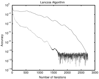
Figure 1. Normalized recursive residual (solid line) and relative differences of (2.18) (dotted line) produced by Algorithm 4.

To illustrate this situation I give an example from a lattice calculation (The lattice size and parameters are given in section 5.1). I compute the bilinear form (2.2) for:

(2.19) $$f(s)=\log\tanh\sqrt{s},~{}~{}~{}~{}~{}s\in\mathbb{R}^{+}$$

and $A=H_{W}^{2}$, $b\in\mathbb{C}^{N}$. The real and imaginary parts of the $b-$elements are chosen randomly from the set $\{+1,-1\}$.

In Fig. 1 are shown the normalized recursive residuals $\rho_{0}/\rho_{i}=\left\|b-Ax_{i}\right\|_{2}/\left\|b\right\|_{2},i=1,\ldots,n$ and relative differences of (2.18) between two successive Lanczos steps. The figure illustrates clearly the different regimes of convergence for the linear system and the bilinear form. The relative differences of the bilinear form converge faster than the computed recursive residual. This example indicates that a stopping criterion based on the solution of the linear system may indeed be strong. Therefore, the recommended stopping criteria would be to monitor the relative differences of the bilinear form but less frequently than proposed by [Bai et al, 1996]. More investigations are needed to settle this issue. Note also the roundoff effects (see Fig. 1) in the convergence of the bilinear form.

3. Conclusion

In this paper I have described computational methods needed to evaluate the effective action of the theory with suppressed cutoff modes.

All methods described in this paper have a complexity that does not depend on the input sparse matrix that describes the fermion theory on the lattice. In this way, it may be concluded that simulation algorithms of lattice QCD which are based on the estimation of the effective fermion action have the same complexity. The UV-suppressed fermions are such an example.

References

- [Bai et al, 1996] Z. Bai, M. Fahey, and G. H. Golub, Some large-scale matrix computation problems, J. Comp. Appl. Math., 74:71-89, 1996.
- [Boriçi, 2002] A. Boriçi, Lattice QCD with Suppressed High Momentum Modes of the Dirac Operator, hep-lat/0205011.
- [Boriçi, 1999b] A. Boriçi, On the Neuberger overlap operator, Phys. Lett. B453 (1999) 46-53
- [Boriçi, 2000a] A. Boriçi, Fast methods for computing the Neuberger Operator, in A. Frommer et al (edts.), Numerical Challenges in Lattice Quantum Chromodynamics, Springer Verlag, Heidelberg, 2000.
- [Boriçi, 2000b] A. Boriçi, A Lanczos approach to the Inverse Square Root of a Large and Sparse Matrix, J. Comput. Phys. 162 (2000) 123-131 and hep-lat/9910045
- [Cahill et al, 1999] E. Cahill, A. Irving, C. Johnson, J. Sexton, Numerical stability of Lanczos methods, Nucl. Phys. Proc. Suppl. 83 (2000) 825-827
- [Duncan, Eichten and Thacker, 1999] A. Duncan, E. Eichten, H. Thacker, An Efficient Algorithm for QCD with Light Dynamical Quarks, Phys. Rev. D59 (1999) 014505
- [de Forcrand, 1999] Ph. de Forcrand, UV-filtered fermionic Monte Carlo, Nucl. Phys. Proc. Suppl. 73 (1999) 822-824
- [Freund, 1993] R. W. Freund, Solution of Shifted Linear Systems by Quasi-Minimal Residual Iterations, in L. Reichel and A. Ruttan and R. S. Varga (edts), Numerical Linear Algebra, W. de Gruyter, 1993
- [Frommer et al, 1995] A. Frommer, S. Güsken, T. Lippert, B. Nöckel and K. Schilling, Many Masses on One Stroke: Economic Computation of Quark Propagators, Int. J. Mod. Phys. C6 (1995) 627-638 and hep-lat/9504020
- [Golub & Van Loan, 1989] G. H. Golub and C. F. Van Loan, Matrix Computations, The Johns Hopkins University Press, Baltimore, 1989
- [Golub & Strakos, 1994] G. H. Golub and Z. Strakos, Estimates in quadratic formulas, Numerical Algorithms, 8 (1994) pp. 241-268.
- [A. Hasenfratz & Knechtli, 2001] A. Hasenfratz and F. Knechtli, Simulating dynamical fermions with smeared links, Nucl. Phys. Proc. Suppl. 106 (2002) 1058-1060. See also A. Hasenfratz, Dynamical Simulation of Smeared Link Actions, Talk given at Lattice 2002, Boston, MA, USA.
- [Irving et al, 1998] A. C. Irving, J. C. Sexton, E. Cahill, J. Garden, B. Joo, S. M. Pickles, Z. Sroczynsk , Tuning Actions and Observables in Lattice QCD, Phys. Rev. D58 (1998) 114504
- [B.Jegerlehner, 1998] B. Jegerlehner, Multiple mass solvers, Nucl. Phys. Proc. Suppl. 63 (1998) 958-960
- [Lanczos, 1952] C. Lanczos, Solution of systems of linear equations by minimized iterations, J. Res. Nat. Bur. Stand., 49 (1952), pp. 33-53
- [Peardon, Lattice2001] M. Peardon, Progress in lattice algorithms Nucl. Phys. B (Proc.Suppl.) 106&107 (2002) 3-11. See also M. Peardon, Multiple molecular dynamics time-scales in Hybrid Monte Carlo fermion simulations, Talk given at Lattice 2002, Boston, MA, USA.
- [Press et al, 1993] W.H. Press, S.A. Teukolsky, W.T. Vetterling, B.P. Flannery, Numerical Recipes in FORTRAN, Cambridge University Press, 1993