We investigate spectral functions extracted using the Maximum Entropy Method from correlators measured in lattice simulations of the (2+1)-dimensional four-fermion model. This model is particularly interesting because it has both a chirally broken phase with a rich spectrum of mesonic bound states and a symmetric phase where there are only resonances. In the broken phase we study the elementary fermion, pion, sigma, and massive pseudoscalar meson; our results confirm the Goldstone nature of the $\pi$ and permit an estimate of the meson binding energy. We have, however, seen no signal of $\sigma\to\pi\pi$ decay as the chiral limit is approached. In the symmetric phase we observe a resonance of non-zero width in qualitative agreement with analytic expectations; in addition the ultra-violet behaviour of the spectral functions is consistent with the large non-perturbative anomalous dimension for fermion composite operators expected in this model.

1 Introduction

The Gross-Neveu model in $d=3$ spacetime dimensions (GNM₃) has been the object of much analytic and numerical study in recent years. Its Lagrangian density is

$${\cal L} = \bar{\psi}_{i}(\partial\hskip-5.0pt/+m)\psi_{i}-\frac{g^{2}}{2N_{f}}[(\bar{\psi}_{i}\psi_{i})^{2}-(\bar{\psi}_{i}\gamma_{5}\psi_{i})^{2}]$$ (1.1)

$$\sim \bar{\psi}_{i}\biggl{(}\partial\hskip-5.0pt/+m+{g\over\surd N_{f}}(\sigma+i\gamma_{5}\pi)\biggr{)}\psi_{i}+\frac{1}{2}(\sigma^{2}+\pi^{2}),$$ (1.2)

where the index $i$ runs over $N_{f}$ fermion flavors and in the second line we have introduced scalar $\sigma$ and pseudoscalar $\pi$ auxiliary boson fields. Apart from the obvious numerical advantages of working with a relatively simple theory in a reduced dimensionality there are several features which make GNM₃ interesting for the modelling of strong interactions [1].

• For sufficiently strong coupling $g^{2}>g_{c}^{2}$ it exhibits spontaneous chiral symmetry breaking implying dynamical generation of a fermion mass $M_{f}$, the pion field $\pi$ being the associated Goldstone boson. A separation of scales $m_{\pi}\ll M_{f}$ is possible.

• The spectrum of excitations contains both “baryons” and “mesons”, namely the elementary fermions $f$ and the composite $f\bar{f}$ states;

• For $2<d<4$ there is an interacting continuum limit at a critical value of the coupling, which for $d=3$ has a numerical value $g_{c}^{2}/a\approx 1.0$ in the large-$N_{f}$ limit if a lattice regularisation is employed [2]. There is a renormalisation group UV fixed point at $g^{2}=g_{c}^{2}$, signalled by the renormalisability of the $1/N_{f}$ expansion [1], entirely analagous to the Wilson-Fisher fixed point in scalar field theory.

• Numerical simulations with baryon chemical potential $\mu\not=0$ show qualitatively correct behaviour, in that the onset of matter occurs for $\mu$ of the same order as the constituent quark scale $M_{f}$ [3], rather than for $\mu\approx m_{\pi}/2$, which happens in gauge theory simulations with a real measure $\mbox{det}(M^{\dagger}M)$ because of the presence of a baryonic pion in the spectrum. This makes GNM₃ an ideal arena in which to test strongly interacting thermodynamics [4].

Let us briefly review the physical content of the model as predicted by the large-$N_{f}$ approach [1, 2]. For $g^{2}>g_{c}^{2}$ the fermion has a dynamically generated mass $M_{f}$ given, up to corrections of order $1/N_{f}$, by

$$M_{f}={g\over\surd N_{f}}\langle\sigma\rangle={g^{2}\over N_{f}}\langle\bar{\psi}\psi\rangle.$$ (1.3)

Its inverse defines a correlation length which diverges as $(g^{2}-g_{c}^{2})^{-\nu}$ with critical index $\nu=1+O(1/N_{f})$. In addition as a result of $f\bar{f}$ loop corrections the $\sigma$ and $\pi$ fields acquire non-trivial dynamics, the inverse $\sigma$ propagator being given as a function of $d$ to leading order in $1/N_{f}$ by

$$D_{\sigma}(k^{2})={1\over g^{2}}{{(4\pi)^{d\over 2}}\over{2\Gamma(2-{\textstyle{d\over 2}})}}{M_{f}^{4-d}\over{(k^{2}+4M_{f}^{2})F(1,2-{\textstyle{d\over 2}};{3\over 2};-{k^{2}\over{4M_{f}^{2}}})}}.$$ (1.4)

Immediately we see the difference between this model and QCD. For $k^{2}\ll M_{f}^{2}$ $F\approx 1$, implying that to this order the $\sigma$ resembles a weakly-bound meson of mass $M_{\sigma}=2M_{f}$; however, the hypergeometric function in the denominator indicates a strongly interacting $f\bar{f}$ continuum immediately above the threshold $2M_{f}$. This implies that if truly bound, its binding energy is $O(1/N_{f})$ at best (to our knowledge there have so far been no analytic calculations), implying little if any separation between pole and threshold. Since all residual interactions are subleading in $1/N_{f}$, we surmise that all other mesons are similarly weakly bound states of massive fermions, and hence effectively described by a two-dimensional “non-relativistic quark model”. A recent study of mesonic wavefunctions in GNM₃ provides evidence for this picture [5]. In an asymptotically-free but confining theory like QCD, by contrast, one expects isolated poles and/or resonances, corresponding to relativistic bound states in the channel in question, which are well separated from a threshold to nearly-free quark behaviour which sets in at typically 1.3 - 1.5 GeV [6].

The exception to this rule is the pion. The Lagrangian (1.2) can be defined with either a continuous U(1) or discrete Z₂ chiral symmetry, the latter case being realised by setting the $\pi$ field to zero. In the case of U(1) chiral symmetry, for $m=0$ and $g^{2}>g_{c}^{2}$ the pion propagator $D_{\pi}$ is given by a similar expression to (1.4) with the factor $(k^{2}+4M_{f}^{2})$ replaced by $k^{2}$; the massless pole demonstrates that $\pi$ couples to a Goldstone mode. For $m>0$, we expect by the usual PCAC arguments that the $\pi$ acquires a mass $m_{\pi}\propto\surd m$, and that the ratio $m_{\pi}/M_{f}$ can be tuned to be arbitrarily small. In particular, once it is less than unity the $\sigma$ becomes unstable with respect to decay into $2\pi$. Note, however, that the Goldstone mechanism in GNM₃ is fundamentally different from that in QCD. In GNM₃ the diagrams responsible for making the pion light are flavor-singlet chains of disconnected $f\bar{f}$ bubbles [3]. The non-singlet connected $f\bar{f}$ diagram which interpolates the pion in QCD corresponds in GNM₃ to a pseudoscalar state with mass $O(2M_{f})$.

For $g^{2}<g_{c}^{2}$ the model is chirally symmetric, and hence all states are massless, as $m\to 0$. In this limit $D_{\sigma}$ and $D_{\pi}$ coincide, and in the large-$N_{f}$ limit neither has a pole on the physical sheet [1]. The auxiliary fields in this case do not interpolate to a stable particle. A dimensionful scale is still defined, however, by the width $\mu$ of a resonance in $f\bar{f}$ scattering in these channels; this diverges as $(g^{2}_{c}-g^{2})^{-\nu}$ with the same exponent $\nu$ [2].

It is clear that despite its simplicity GNM₃ exhibits phenomena such as resonances, decays and multi-particle continua which are not easily analysed using the traditional techniques of single- and multi-exponential fitting to Euclidean correlators developed for quenched QCD. This was recognised in early studies, which attempted fits inspired by the large-$N_{f}$ forms of $D_{\sigma}$ in both chirally broken and symmetric phases, with ambiguous results [2]. A more systematic approach, however, is to focus on the spectral density function $\rho(\omega)$, defined implicitly via the Euclidean timeslice meson correlator $C(t)$ by

$$C(t)=\sum_{\vec{x}}\langle J(\vec{0},0)J^{\dagger}(\vec{x},t)\rangle=\int_{0}^{\infty}d\omega\rho(\omega)e^{-\omega t}.$$ (1.5)

Here $J$ is a local fermion bilinear $\bar{\psi}\Gamma\psi$ which in principle projects onto all physical states consistent with a given set of quantum numbers. All information about bound states, resonances and particle production thresholds as a function of energy $\omega$ is contained in $\rho$. The procedures for fitting lattice-generated data to date have assumed Ansätze for $\rho$ such as one or more bound state poles of the form $\delta(\omega-M)$, or perhaps a free particle continuum above some threshold [7]. However, more recent works have attempted ab initio calculations of $\rho(\omega)$ [8, 9, 10]. This is a difficult problem: the inversion of (1.5) is ill-posed since $\rho(\omega)$ is a continuous function whereas lattice simulations only yield $C(t)$ for a discrete, finite set of points, and moreover with some statistical uncertainty. The approach adopted in Refs. [9] is to apply the Maximum Entropy Method (MEM) which attempts to fit $\rho(\omega)$ subject to reasonable assumptions of smoothness and stability with respect to small variations in the input data.

In this paper we present results from a study of spectral functions extracted from numerical simulations of GNM₃ using MEM techniques. To our knowledge this is the first such study beyond the quenched approximation. Our goal is to explore some of the features described above which distinguish GNM₃ from quenched QCD. In this regard it is worth noting that because the two most important mesonic channels, $\sigma$ and $\pi$, are represented by bosonic auxiliary fields, the correlation functions in these channels automatically include the disconnected diagrams which are so expensive to calculate in QCD; in GNM₃, by contrast, these can be measured with high statistics relatively cheaply. We will also examine the fermion and non-singlet pseudoscalar (PS) channels. As surveyed above, simulations of GNM₃ offer the freedom to vary the phase of the theory (by varying $\mbox{sgn}(g^{2}-g_{c}^{2})$), the correlation length (by varying $|g^{2}-g_{c}^{2}|$), the symmetry group (by including or omitting $\pi$), the ratio $m_{\pi}/M_{f}$ (by varying $m$), and the interaction strength (by varying $N_{f}$) – in the current study we will exploit most of these opportunities. In future work we plan also to study the model with both non-zero temperature $T$ and baryon chemical potential $\mu$.

In Sec. 2 we survey MEM and explain our implementation of it. Sec. 3 outlines some theoretical expectations related to $\rho(\omega)$ in GNM₃ based on the large-$N_{f}$ approach, and Sec. 4 details the lattice formulation and numerical simulations. Our results are presented in Sec. 5, and conclusions in Sec. 6.

2 The Maximum Entropy Method

The theoretical basis for MEM is Bayes’ theorem in probability theory [11]:

$$P[X|Y]=\frac{P[Y|X]P[X]}{P[Y]},$$ (2.1)

where $P[X|Y]$ denotes the conditional probability of $X$ given $Y$. In terms of the lattice data $D$, spectral function $\rho$ and all a priori knowledge $H$, Bayes’ theorem reads:

$$P[\rho|DH]=\frac{P[D|\rho H]P[\rho|H]}{P[D|H]}.$$ (2.2)

$P[D|\rho H]$ is known as the likelihood function and is the equivalent of the familiar $\chi^{2}$ in the least squares method [12]. For a large number of Monte Carlo measurements of a correlation function, the data $D$ are expected to obey a gaussian distribution according to the central limit theorem,

$$P[D|\rho H] = \frac{1}{Z_{L}}e^{-L[\rho]},$$ (2.3)

$$L[\rho] = \frac{1}{2}\sum_{i,j=1}^{N_{t}}(D(t_{i})-D_{\rho}(t_{i}))C_{ij}^{-1}(D(t_{j})-D_{\rho}(t_{j})),$$ (2.4)

where the normalisation factor $Z_{L}=(2\pi)^{\frac{N_{t}}{2}}\sqrt{\det C}$ and $N_{t}$ is the number of temporal points. Lattice data averaged over $N_{\rm cfg}$ gauge configurations $D(t)$, the covariance matrix $C_{ij}$, and the propagator constructed from the spectral function $\rho$ using the lattice kernel $K(\omega,t)$ are defined by

$$D(t_{i}) = \frac{1}{N_{\rm cfg}}\sum_{m=1}^{N_{\rm cfg}}D^{m}(t_{i}),$$ (2.5)

$$C_{ij} = \frac{1}{N_{\rm cfg}(N_{\rm cfg}-1)}\sum_{m=1}^{N_{\rm cfg}}(D^{m}(t_{i})-D(t_{i}))(D^{m}(t_{j})-D(t_{j})),$$ (2.6)

$$D_{\rho}(t) = \int_{0}^{\infty}K(t,\omega)\rho(\omega)d\omega.$$ (2.7)

In all our work we use a lattice kernel defined as $\exp(-\omega t)$.

The factor $P[\rho|H]$ appearing in the numerator of (2.2) is the prior probability, which is written in terms of the Shannon-Jaynes entropy $S[\rho]$ [13] for a given default model $\rho_{0}(\omega)$. The default model is usually chosen to be the spectral function for a non-interacting two-particle continuum; for meson states we have $\rho_{0}(\omega)\propto\omega^{d-2}$ (see Sec. 3). The final result, however, should be insensitive to the choice of $\rho_{0}$. The entropy $S[\rho]\leq 0$ and becomes zero only when $\rho(\omega)=\rho_{0}(\omega)$:

$$P[\rho|H\alpha\rho_{0}] = \frac{1}{Z_{S}(\alpha)}e^{\alpha S[\rho]},$$ (2.8)

$$S[\rho] = \int_{0}^{\infty}\left[\rho(\omega)-\rho_{0}(\omega)-\rho(\omega)\ln\left(\frac{\rho(\omega)}{\rho_{0}(\omega)}\right)\right]d\omega$$ (2.9)

$$\rightarrow \sum_{\ell=1}^{N_{\omega}}\left[\rho_{\ell}-\rho_{0\ell}-\rho_{\ell}\ln\left(\frac{\rho_{\ell}}{\rho_{0\ell}}\right)\right]\Delta\omega,$$ (2.10)

where Eq. (2.10) results from discretising the $\omega$-axis into $N_{\omega}$ bins of width $\Delta\omega$, and the normalisation factor $Z_{S}\cong(\frac{2\pi}{\alpha})^{\frac{N_{\omega}}{2}}$. Note that two extra parameters previously implicit in $H$ have been written in explicitly; $\alpha$ is a real positive parameter and $\rho_{0}(\omega)$ a real positive function. This form of entropy leads to a positive semi-definite spectral function in MEM. In our work we use $N_{\omega}=600$ and $\Delta\omega a=0.01$.

Combining Eqs. (2.3) and (2.8) gives

$$P[\rho|DH\alpha\rho_{0}] \propto \frac{1}{Z_{S}Z_{L}}e^{Q[\rho]},$$ (2.11)

$$Q \equiv \alpha S-L.$$ (2.12)

and the condition satisfied by the most probable spectral function $\rho_{\alpha}(\omega)$ is

$$\left.\frac{\delta Q}{\delta\rho(\omega)}\right|_{\rho=\rho_{\alpha}}=0$$ (2.13)

The parameter $\alpha$ is in effect a relative weighting between the entropy $S$ and the likelihood $L$, and there are three different ways to deal with it. The value $\alpha=\hat{\alpha}$ can be chosen which either gives $\chi^{2}=N_{t}$ or maximises $P[\alpha|DH\rho_{0}]$; these methods are known as classic and historic [13] respectively. Alternatively, a weighted average over $P[\alpha|DH\rho_{0}]$ can be performed; this is known as Bryan’s method [14] and is the one we adopt:

$$\rho_{out}(\omega)=\int_{\alpha_{min}}^{\alpha_{max}}d\alpha\rho_{\alpha}(\omega)P[\alpha|DH\rho_{0}],$$ (2.14)

where $\alpha_{min}$ and $\alpha_{max}$ are chosen to satisfy

$$P[\alpha_{min,max}|DH\rho_{0}]=0.01P[\hat{\alpha}|DH\rho_{0}].$$ (2.15)

2.1 Testing MEM

To test our implementation of MEM, we studied an idealised QCD spectral function in the charged $\rho$-meson channel [6, 8]:

$${\rho_{in}(\omega)\over\omega^{2}}=\frac{2}{\pi}\left[F_{\rho}^{2}\frac{\Gamma_{\rho}m_{\rho}}{(\omega^{2}-m_{\rho}^{2})^{2}+\Gamma_{\rho}^{2}m_{\rho}^{2}}+\frac{1}{8\pi}(1+\frac{\alpha_{s}}{\pi})\frac{1}{1+e^{(\omega_{0}-\omega)/\delta}}\right],$$ (2.16)

where the pole residue $F_{\rho}=f_{\rho}m_{\rho}$ is defined by

$$\langle 0|\bar{d}\gamma_{\mu}u|\rho\rangle\epsilon_{\mu}=\sqrt{2}f_{\rho}m_{\rho}^{2}\epsilon_{\mu},$$ (2.17)

$\epsilon_{\mu}$ being the polarisation vector. The following energy-dependent width is chosen with a $\theta$-function included to give the correct threshold behaviour of the $\rho\rightarrow\pi\pi$ decay

$$\Gamma_{\rho}(\omega)=\frac{g_{\rho\pi\pi}^{2}}{48\pi}m_{\rho}\left(1-\frac{4m_{\pi}^{2}}{\omega^{2}}\right)^{3/2}\theta(\omega-2m_{\pi}).$$ (2.18)

The values of the parameters input into (2.16) are taken to be:

$$m_{\rho}=0.77,\;\;m_{\pi} = 0.14,\;\;\omega_{0}=1.3,$$ (2.19)

$$g_{\rho\pi\pi}=5.45,\;\;f_{\rho} = 0.184,\;\;\delta=0.2,\;\;\alpha_{s}=0.3.$$ (2.20)

where the numerical values of the first three parameters are in GeV.

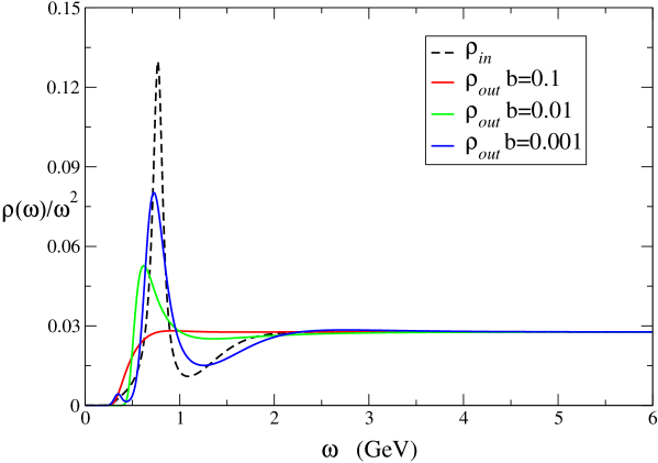
Figure 1: Comparison of $\rho_{in}$ and $\rho_{out}$ for idealised data in the $\rho$-channel with $N_{t}=32$.

Test lattice correlator data were constructed from the spectral function using (2.7). Gaussian noise with variance $\sigma(t_{i})=bD_{in}(t_{i})t_{i}$ was added to this data to simulate the effect of decreasing signal-to-noise ratio with temporal separation [8]. For simplicity we use a diagonal covariance matrix, which thus neglects correlations between different $t$. The default model used is $\rho_{0}(\omega)=m_{0}\omega^{2}$, motivated by the asymptotic behaviour of $\rho_{in}$. The parameter $m_{0}$ is chosen to be $\lim_{\omega\to\infty}\rho_{in}(\omega)=0.0277$. We set $\omega_{max}=6$GeV, $\Delta\omega=10$MeV and $N_{\omega}=600$, and vary the noise parameter $b$ from 0.1 to 0.001. Fig. 1 shows a comparison between $\rho_{in}$ and $\rho_{out}$ for various $b$. As expected, decreasing $b$ leads to a better agreement between input and output spectral functions.

3 Theoretical Preliminaries

Our main focus will be the mesonic Euclidean timeslice correlation functions defined in Eqn. (1.5). With this definition, if $J$ couples to a stable (ie. zero width) bound state of mass $M$ with strength $A$ (ie. $\langle 0|J|\vec{k},M\rangle=A$), then $\rho(\omega)=(|A|^{2}/2M)\delta(\omega-M)$. Since in $d$ spacetime dimensions the engineering dimension $[J]=d-1$ and $[|\vec{k},M\rangle]=1-{d\over 2}$, it is readily checked that the combination $\rho(\omega)/\omega^{d-2}$ is dimensionless. This also motivates the use of the default model $\rho_{0}(\omega)\propto\omega^{d-2}$, which corresponds in configuration space to the propagation of free massless fermions; ie. $C(t)\propto t^{-(d-1)}$. For an asymptotically-free theory such as QCD we expect $\lim_{\omega\to\infty}\rho(\omega)=\rho_{0}(\omega)$, as illustrated in Fig. 1: however since GNM₃’s UV behaviour is described by a renormalisation group fixed point with non-vanishing interaction strength [1, 2] this is not a constraint in the current study.

The asymptotic form of $\rho(\omega)$ is easiest to analyse in the symmetric phase $g^{2}<g_{c}^{2}$ of the model, where we have a large-$N_{f}$ prediction [15, 2]. In the scalar channel, the momentum space propagator

$$D_{\sigma}(k^{2})\propto{{\mu^{d-2}}\over{(\surd k^{2})^{d-2}+\mu^{d-2}}}$$ (3.1)

where $2<d<4$ and $\mu$ is a dimensionful scale which increases as $(g_{c}^{2}-g^{2})^{1\over{d-2}}$, ie. as an inverse correlation length. For $d=3$ this implies [16]

$$C_{\sigma}(t)\propto\mu\int_{0}^{\infty}dk{{\cos kt}\over{k+\mu}}\equiv\mu\int_{0}^{\infty}d\omega{\omega\over{\omega^{2}+\mu^{2}}}e^{-\omega t},$$ (3.2)

and hence the large-$N_{f}$ prediction

$$\rho_{\sigma}(\omega)\propto{{\mu\omega}\over{\omega^{2}+\mu^{2}}}.$$ (3.3)

In the asymptotic regime we thus have $\rho_{\sigma}\to\rho_{UV}(\omega)\propto\omega^{-1}$ rather than $\rho_{0}(\omega)\propto\omega$. This is a consequence of the large non-perturbative anomalous dimension $\eta_{\bar{\psi}\psi}=d-2$ acquired by the scalar density at the UV fixed point [2], which relates the asymptotic forms via

$$\rho_{UV}(\omega)\propto\rho_{0}(\omega)\omega^{-2\eta_{\bar{\psi}\psi}}.$$ (3.4)

At smaller energy scales we interpret $\rho$ as describing a resonance whose central position and width are both $O(\mu)$ and hence increase as the coupling $g^{2}$ is reduced. A second prediction of (3.3) is that the dimensionless combination $\rho(\omega)/\omega$ tends to a constant in the IR limit $\omega\to 0$.

Another situation of interest is the possibility of $\sigma$ decay in the chirally broken phase. Denote the physical fermion mass by $M_{f}$; the $\sigma$ is then expected to be a weakly bound state of mass $M_{\sigma}\raisebox{-2.15277pt}{$\ \stackrel{{\scriptstyle\textstyle<}}{{\textstyle\sim}}\ $}2M_{f}$ whereas, for the case of a continuous chiral symmetry, the pion mass $m_{\pi}$ may be much smaller. If $2m_{\pi}<M_{\sigma}$, the decay $\sigma\to 2\pi$ is allowed and should show up as a threshold in the scalar spectral function. This should be a good warm-up exercise for studying the physical decay $\rho\to 2\pi$ in QCD; as well as the computational saving, an important technical consideration in the present case is that unlike in QCD the two pions can be produced in a state of zero relative momentum.

Let us first derive an expectation for the form of the threshold using the $1/N_{f}$ expansion. The contribution of the two pion intermediate state to the $\sigma$ correlator is shown diagramatically in Fig. 2.

Figure 2: Contribution to $D_{\sigma}$ from a 2$\pi$ intermediate state.

To leading order in $1/N_{f}$, using the conventions of Sec. 2 of [2] the $\sigma$ propagator is given by Eqn. (1.4) where for momenta $k\ll M_{f}$ the hypergeometric function in the denominator may be approximated by $F\approx 1$. We will assume that for bare fermion mass $m>0$, the pion propagator $D_{\pi}$ is given by the same expression with the factor $(k^{2}+4M_{f}^{2})$ in the denominator replaced by $(k^{2}+m_{\pi}^{2})$. The vertex $\Gamma_{\sigma\pi\pi}$ is assumed to arise from a single fermion loop as indicated in Fig. 2. It is identically zero if chiral symmetry is unbroken. Using the bare vertex $-g/\surd N_{f}$, it is straightforward to show

$$\Gamma_{\sigma\pi\pi}\simeq-G_{\sigma\pi\pi}{{g^{3}M_{f}^{d-3}}\over{\surd N_{f}}}$$ (3.5)

where $G_{\sigma\pi\pi}$ is a dimensionless $d$-dependent constant.

With these components in place it is now possible to calculate $D_{\sigma}$ including the effects of the two pion intermediate state. Specialising to $d=3$, we find

$$D_{\sigma}^{-1}(k^{2}\ll M_{f}^{2})={g^{2}\over{4\pi M_{f}}}\left[k^{2}+4M_{f}^{2}-{{G_{\sigma\pi\pi}^{2}}\over N_{f}}{M_{f}^{3}\over{\surd k^{2}}}\tan^{-1}\left({{\surd k^{2}}\over{2m_{\pi}}}\right)\right].$$ (3.6)

Besides the pole at $k^{2}\simeq-4M_{f}^{2}$, there is now a contribution at $O(1/N_{f})$ to the timeslice correlation function given by

$$C_{\sigma}^{(1)}(t)\propto{{G_{\sigma\pi\pi}^{2}M_{f}^{3}}\over N_{f}}\int{{dk}\over{2\pi}}{{e^{ikt}}\over{k(k^{2}+4M_{f}^{2})^{2}}}\tan^{-1}\left({k\over{2m_{\pi}}}\right),$$ (3.7)

The two pion threshold manifests itself via branch cuts in the inverse tangent running from $k^{2}=-4m_{\pi}^{2}$ out to $\pm i\infty$. Approximating $k^{2}\ll M_{f}^{2}$ as before we integrate around the cut in the upper half plane to obtain

$$C_{\sigma}^{(1)}(t)\propto{{G_{\sigma\pi\pi}^{2}}\over{32N_{f}M_{f}}}\int_{2m_{\pi}}^{\infty}{{d\omega}\over\omega}e^{-\omega t}$$ (3.8)

from which we read off

$$\rho_{\sigma}^{(1)}(\omega)\propto{{G_{\sigma\pi\pi}^{2}}\over{32N_{f}M_{f}}}{1\over\omega}\theta(\omega-2m_{\pi}).$$ (3.9)

Eqn. (3.9) predicts that as well as a pole at $\omega\simeq 2M_{f}$, there should also be a spectral feature at $\omega=2m_{\pi}$ whose strength scales as $(N_{f}M_{f}m_{\pi})^{-1}$; this is in principle testable by varying the simulation parameters $N_{f}$, $g^{2}$ and $m$. On a finite volume it will, however, prove difficult to study the detailed form of the spectral function above threshold. This is because the number of modes into which the $\sigma$ can decay is strictly delimited by the allowed pion wavevectors $\vec{k}_{\pi}=2\pi\vec{n}/L_{s}$, where $\vec{n}$ has integer-valued components, and $2\sqrt{m_{\pi}^{2}+k_{\pi}^{2}}<M_{\sigma}$. The optical theorem, however, implies that the only intermediate states which can contribute to $\rho(\omega)$ are possible decay modes of the $\sigma$; we infer that on a finite lattice, the $\omega^{-1}$ shape predicted by (3.9) is replaced by a set of $\delta$-functions, each arising from an allowed $\vec{k}_{\pi}$. With imperfect (ie. finite) statistical data, however, it is possible that under MEM these isolated poles will blend into a continuum of approximately the correct shape.

4 Simulations

The fermionic part of the lattice action we have used for the semi-bosonized GNM₃ with $U(1)$ chiral symmetry is given by [3]

$$S_{fer} = \bar{\chi}_{i}(x)M_{ijxy}\chi_{j}(y)$$ (4.1)

$$= \sum_{i=1}^{N}\left(\sum_{x,y}\bar{\chi}_{i}(x)\mathcal{M}_{xy}\chi_{i}(y)+\frac{1}{8}\sum_{x}\bar{\chi}_{i}(x)\chi_{i}(x)[\sum_{\langle\tilde{x},x\rangle}\sigma(\tilde{x})+i\epsilon(x)\sum_{\langle\tilde{x},x\rangle}\pi(\tilde{x})]\right),$$

where $\chi_{i}$ and $\bar{\chi}_{i}$ are Grassmann-valued staggered fermion fields defined on the lattice sites, the auxiliary fields $\sigma$ and $\pi$ are defined on the dual lattice sites, and the symbol $\langle\tilde{x},x\rangle$ denotes the set of 8 dual lattice sites $\tilde{x}$ surrounding the direct lattice site $x$. The fermion kinetic operator $\mathcal{M}$ is given by

$$\mathcal{M}_{x,y}=\frac{1}{2}\sum_{\nu}\eta_{\nu}(x)\left[\delta_{y,x+\hat{\nu}}-\delta_{y,x-\hat{\nu}}\right]+m\delta_{x,y},$$ (4.2)

where $\eta_{\nu}(x)$ are the Kawamoto-Smit phases $(-1)^{x_{0}+\cdots+x_{\nu-1}}$, and the symbol $\epsilon(x)$ denotes the alternating phase $(-1)^{x_{0}+x_{1}+x_{2}}$. The auxiliary fields $\sigma$ and $\pi$ are weighted in the path integral by an additional factor corresponding to

$$S_{aux}=\frac{N}{2g^{2}}\sum_{\tilde{x}}[\sigma^{2}(\tilde{x})+\pi^{2}(\tilde{x})].$$ (4.3)

The simulations were performed using a standard hybrid Monte Carlo (HMC) algorithm without even/odd partioning, implying that simulation of $N$ staggered fermions describes $N_{f}=4N$ continuum species [3]; the full symmetry of the lattice model in the continuum limit, however, is $U(N_{f}/2)_{V}\otimes U(N_{f}/2)_{V}\otimes U(1)$ rather than $U(N_{f})_{V}\otimes U(1)$. At non-zero lattice spacing the symmetry group is smaller still: $U(N_{f}/4)_{V}\otimes U(N_{f}/4)_{V}\otimes U(1)$. In the $Z_{2}$-symmetric model the $\pi$ fields are switched off and $M$ becomes real so that real pseudofermion fields can be used. In this case $N$ staggered fermions describe $N_{f}=2N$ continuum species. Further details of the algorithm and the optimisation of its performance can be found in [2, 3].

Using point sources we calculated the zero momentum fermion $(f)$ correlator at different values of the coupling $\beta\equiv 1/g^{2}$. In order to compare MEM to conventional spectroscopy we also estimated the fermion mass using a simple pole fit using the function

$$C_{f}(t)=A_{f}[e^{-M_{f}t}-(-1)^{t}e^{-M_{f}(L_{t}-t)}].$$ (4.4)

Similarly, the zero momentum auxiliary $\pi$ correlator was measured and its mass estimated using a cosh fit. The mesonic correlators are given by:

$$C_{M}(t)=\sum_{\mathbf{x},\bf{x}_{1},\mathbf{x}_{2}}\Phi(\mathbf{x}_{1})\Phi(\mathbf{x}_{2})W_{M}({\mathbf{x}})G(\mathbf{x},t;\mathbf{x}_{1},0)G^{\dagger}(\mathbf{x},t;\mathbf{x}_{2},0),$$ (4.5)

where $G$ is the lattice fermion propagator and $W_{M}({\mathbf{x}})$ a phase factor which picks out a channel with particular symmetry properties i.e. $W_{M}({\mathbf{x}})=\epsilon(x)$ for the S channel and $W_{M}({\mathbf{x}})=1$ for the PS channel. The function $\Phi(\mathbf{x})$ is either a point source $\delta_{\mathbf{x},(0,0)}$ or a staggered fermion wall source $\sum_{m,n=0}^{L_{s}/2-1}\delta_{\mathbf{x},(2m,2n)}$ [17]. In all the simulations we used point sinks. These correlators were fitted to a function $C_{M}(t)$ given by

$$C_{M}(t)=A[e^{-M_{M}t}+e^{-M_{M}(L_{t}-t)}]+\tilde{A}(-1)^{t}[e^{-\tilde{M}_{M}t}+e^{-\tilde{M}_{M}(L_{t}-t)}].$$ (4.6)

Note that composite operators made from staggered fermion fields project onto more than one set of continuum quantum numbers. The first square bracket represents the “direct” signal with mass $M_{M}$ and the second an “alternating” signal with mass $\tilde{M}_{M}$. Continuum quantum numbers for various mesonic channels are given in [5] – in this study we focus on the PS_direct channel, with $J^{P}=0^{-}$. Although expected to be the tightest bound meson since it is the only one for which $s$-wave binding is available, as stressed in [3, 5] this state does not project onto the Goldstone mode in the broken phase.

5 Results

5.1 The $\pi$, $f$ and PS Channels in the Broken Phase

Figure 3: Propagators in three different channels from simulations of the U(1) model on a $32^{2}\times 48$ lattice at $\beta=0.55$, $m=0.01$.

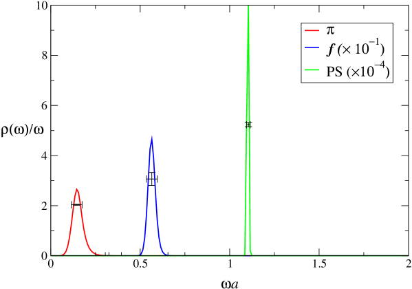
Figure 4: Bryan image of $\rho(\omega)/\omega$ in three different channels using the same data as Fig. 3.

We first discuss results from the chirally broken phase, obtained with $\beta<\beta_{c}\approx 1.0$. Fig. 3 shows the propagators for $\pi$, $f$ and PS channels on a log scale (using data obtained with a wall source and point sink in the latter case), resulting from approximately 40000 HMC trajectories of mean length 1.0. All three look to be well-approximated by straight lines, implying that each channel is dominated by a single particle pole. Fig. 4 shows the spectral functions obtained in the same three channels using Bryan’s method. All three appear as well-localised peaks suggesting simple poles and hence stable particle states. The cross shown on each peak is obtained as follows. The spectral feature is fitted to a form $ZG(\omega-M/\Gamma)$ where $G(x)$ is the normalised gaussian distribution, $M$ the peak position, $\Gamma$ the full width at half maximum, and $Z$ a normalisation factor. The horizontal bar’s position and width represent $M$ and $\Gamma$ respectively, and its height represents the area of $ZG(\omega-M/\Gamma)$ evaluated between $\omega-\Gamma$ and $\omega+\Gamma$. The vertical error bar represents the error in this area as determined by the Bryan algorithm [14]. For a narrow gaussian, of course, the central value is interpreted as the particle mass.

	$N_{f}$	Volume	$\beta$	$m$	Mass	Mass	Area
					(1-exp)	(MEM)
$\pi$	4	$32^{2}\times 48$	0.55	0.005	0.114(4)	0.112(6)	0.501(129)
	4	$32^{2}\times 48$	0.55	0.01	0.168(5)	0.154(9)	0.176(15)
	4	$32^{2}\times 48$	0.55	0.02	0.232(5)	0.231(7)	0.0617(98)
	4	$32^{2}\times 48$	0.55	0.03	0.280(10)	0.263(15)	0.0351(37)
	4	$32^{2}\times 48$	0.55	0.045	0.349(8)	0.326(14)	0.0193(15)
	4	$32^{2}\times 48$	0.55	0.06	0.447(24)	0.435(1.9)	0.0102(5.7)
	4	$32^{2}\times 48$	0.65	0.01	0.193(4)	0.187(8)	0.0810(78)
	4	$32^{2}\times 48$	0.65	0.02	0.277(4)	0.267(6)	0.0289(19)
	36	$24^{2}\times 32$	0.55	0.01	0.150(5)	0.144(18)	0.053(19)
	36	$24^{2}\times 32$	0.55	0.02	0.238(6)	0.229(8)	0.0140(14)
	36	$24^{2}\times 32$	0.55	0.03	0.287(10)	0.271(17)	0.0081(10)
$f$	4	$32^{2}\times 48$	0.55	0.005	0.555(7)	0.556(4)	2.15(49)
	4	$32^{2}\times 48$	0.55	0.01	0.564(1)	0.564(1)	2.37(3)
	4	$32^{2}\times 48$	0.55	0.02	0.5853(7)	0.5858(13)	2.14(27)
	4	$32^{2}\times 48$	0.55	0.03	0.599(1)	0.599(1)	2.06(5)
	4	$32^{2}\times 48$	0.55	0.045	0.623(1)	0.623(1)	1.90(4)
	4	$32^{2}\times 48$	0.55	0.06	0.644(2)	0.643(2)	1.63(8)
	4	$32^{2}\times 48$	0.65	0.01	0.3978(8)	0.3965(13)	5.11(9)
	4	$32^{2}\times 48$	0.65	0.02	0.4285(6)	0.4384(44)	4.10(33)
	36	$24^{2}\times 32$	0.55	0.01	0.6796(3)	0.6796(3)	1.77(8)
	36	$24^{2}\times 32$	0.55	0.02	0.6911(3)	0.6908(3)	1.72(7)
	36	$24^{2}\times 32$	0.55	0.03	0.7025(4)	0.7023(5)	1.59(2)
PS	4	$32^{2}\times 48$	0.55	0.005	1.0807(8)	1.0807(8)	164.3(6)
	4	$32^{2}\times 48$	0.55	0.01	1.0973(8)	1.0979(7)	160(3)
	4	$32^{2}\times 48$	0.55	0.02	1.1395(6)	1.1396(5)	147.2(5)
	4	$32^{2}\times 48$	0.55	0.03	1.1715(11)	1.1716(11)	130(2)
	4	$32^{2}\times 48$	0.55	0.045	1.2253(6)	1.2231(6)	119.1(9)
	4	$32^{2}\times 48$	0.55	0.06	1.2693(13)	1.2691(2)	103(2)
	4	$32^{2}\times 48$	0.65	0.01	0.7722(6)	0.7711(4)	426(32)
	4	$32^{2}\times 48$	0.65	0.02	0.8362(5)	0.8381(45)	343(462)
	36	$24^{2}\times 32$	0.55	0.01	1.3568(2)	1.3569(2)	50.1(3)
	36	$24^{2}\times 32$	0.55	0.02	1.3806(2)	1.3808(2)	48.4(2)
	36	$24^{2}\times 32$	0.55	0.03	1.4030(3)	1.4030(3)	45.5(3)

Table 1: Broken phase spectroscopy

In Table 1 we list the masses obtained from simulations of the U(1) model from both single exponential fits and MEM, as well as the area under the gaussian peak, using correlator data from timeslices 2 – 10 for the $\pi$; for $f$ and PS timeslices 2 – 8 were used. Note that for the lightest state, namely the $\pi$, MEM systematically yields a lower mass, suggesting that it is less affected by excited state contamination, although in all cases the two methods are within a standard deviation.

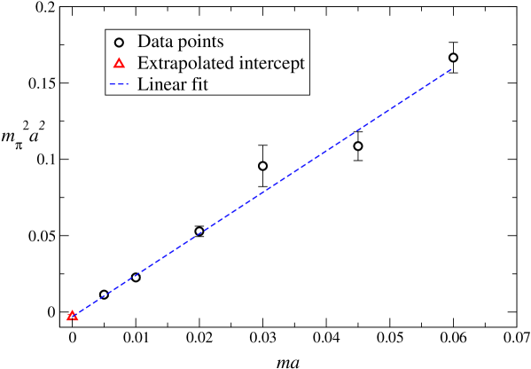
Figure 5: Pion mass $m_{\pi}^{2}$ vs. bare mass $m$ for $\beta=0.55$, showing evidence for the Goldstone nature of the $\pi$.

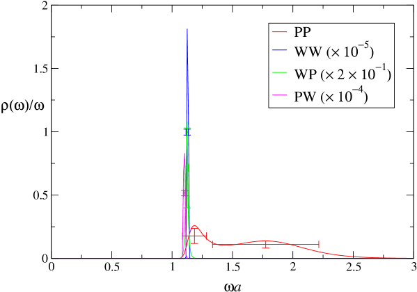
Figure 6: Bryan image of $\rho(\omega)/\omega$ in the PS channel $32^{2}\times 48$ lattice at $\beta=0.55$, $m=0.01$ using correlators with different combinations of wall and point sources.

Fig. 5 demonstrates that the pion mass extracted using MEM over a range of bare fermion masses is consistent with the PCAC behaviour $m_{\pi}\propto\surd m$ expected for broken chiral symmetry. For the $f$ and PS channels there is excellent agreement in almost all cases between the two methods. The PS mass is roughly twice that of the fermion, consistent with its being a weakly bound state. With the precision we have obtained it is possible to estimate the binding energy defined as $\Delta_{M}=2M_{f}-M_{\rm PS}$; the results are tabulated in Table 2.

$N_{f}$	Volume	$\beta$	$m$	$\Delta_{M}$	$\Delta_{M}$
				(1-exp)	(MEM)
4	$32^{2}\times 48$	0.55	0.005	0.0293	0.0313
4	$32^{2}\times 48$	0.55	0.01	0.0307	0.0301
4	$32^{2}\times 48$	0.55	0.02	0.0311	0.0320
4	$32^{2}\times 48$	0.55	0.03	0.0265	0.0264
4	$32^{2}\times 48$	0.55	0.045	0.0207	0.0229
4	$32^{2}\times 48$	0.55	0.06	0.0187	0.0169
4	$32^{2}\times 48$	0.65	0.01	0.0234	0.0219
4	$32^{2}\times 48$	0.65	0.02	0.0208	0.0387
36	$24^{2}\times 32$	0.55	0.01	0.0024	0.0023
36	$24^{2}\times 32$	0.55	0.02	0.0016	0.0008
36	$24^{2}\times 32$	0.55	0.03	0.0020	0.0016

Table 2: Binding Energy in the PS channel

For $N_{f}=4$ $\Delta_{M}\approx 2.8\%$ of the bound state mass, but the figure drops to $\approx 0.15\%$ for $N_{f}=36$, which is roughly consistent with the analytical expectation that $\Delta_{M}\propto 1/N_{f}$ (note, however, that the $N_{f}=36$ simulations were performed on a smaller volume). It was observed in [5] that the PS wavefunction has considerably greater spatial extent for larger $N_{f}$, again implying it is less strongly bound.

As discussed in Sec. 3 the area under the peak is related to the strength $A$ of the coupling of the operator $J$ to the single particle state, and hence to physical decay constants. Our results show a systematic decrease in this coupling strength with bare fermion mass $m$, the effect being most pronounced for the $\pi$.

Finally in Fig. 6 we explore the effects of using different meson sources following Eqn. (4.5) using data from timeslices 1 – 8. As in Fig. 4, the spectral functions have been rescaled so as all to fit on the same plot. When a wall is used at either sink or source, the signal is completely dominated by the bound state; however, for the point-to-point correlator there is a significant contribution out to $\omega a\approx 2.5$. Since we have discarded data from small timeslices we should not expect much quantitative information from the asymptotic form of $\rho(\omega)$ in this case; indeed, as $\omega\to\infty$ it decays much faster than either of the idealised forms $\rho_{0}(\omega)$ or $\rho_{UV}(\omega)$ discussed in Sec. 3. Fig. 6 provides a graphic illustration, however, of the importance of choice of source in maximising the projection onto the ground state.

5.2 Symmetric Phase

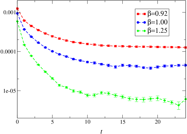
Figure 7: $\sigma$ correlator for 3 different couplings in the chirally symmetric phase on a $32^{2}\times 48$ lattice.

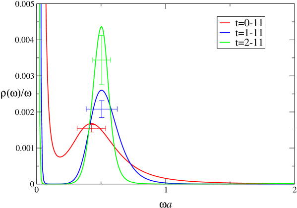
Figure 8: Bryan image of $\rho(\omega)/\omega$ vs. $\omega$ in the $\sigma$ channel at $\beta=1.25$ on a $32^{2}\times 48$ lattice, showing 3 different time windows.

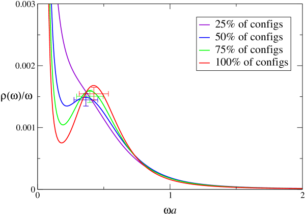
Figure 9: The same as Fig. 8 using fits from timeslices 0 – 11, showing the effects of varying the amount of data.

Next we turn to the chirally symmetric phase found for $\beta>\beta_{c}$, where according to the discussion of Sec. 3 the bound state poles should be replaced by resonances with non-vanishing widths. Our simulations in this section were performed for the Z₂ model on a $32^{2}\times 48$ lattice at couplings $\beta=0.92$, 1.0 and 1.25 with $O(40000)$ configurations separated by HMC trajectories of mean length 1.0, and for U(1) on a $32^{3}$ lattice at $\beta=1.0$ and 1.25 with respectively 30000 and 60000 trajectories of mean length 0.6. In all cases $N_{f}=4$ fermion flavors were used. It proved considerably easier in this phase to simulate the model with Z₂ chiral symmetry: the U(1) simulations required a much smaller molecular dynamics timestep making them more expensive, and the data correspondingly of not such good quality. Data for the Z₂ $\sigma$ timeslice correlator are shown on a log scale in Fig. 7. In contrast to the broken phase correlators of Fig. 3 it is clear that a simple pole fit will not be successful; indeed, the correlators become almost flat at large $t$, which means that towards the centre of the lattice we have to worry about significant contributions from not just a backwards-propagating signal, but also “image” sources displaced by integer mulitples of $L_{t}$ from the original source [2].

If we are to successfully identify spectral features as something other than simple poles, then it is important to study systematic effects. Fig. 8 presents results from the $\sigma$ channel, where the resonance is anticipated, showing the effects of varying the timeslice sample used in the MEM fit. Data from within a time window $[t_{1},t_{2}]$ were fitted; in all cases we chose a rather conservative value $t_{2}=11$ to minimise finite volume (actually non-zero temperature) effects due to the image sources discussed above, although we have checked that the results are insensitive to reducing $t_{2}$. Fig. 8 shows a broad feature centred at $\omega a\simeq 0.5$, whose “width” (actually the ratio of width to area, as indicated by the crosses) increases as data from smaller times is included. Ignoring the divergence as $\omega\to 0$ which we take to be an artifact (possibly due to a small residual vacuum expectation $\langle\sigma\rangle\not=0$; see discussion below in Sec. 5.3), the shape of the spectrum appears qualitatively similar to the large-$N_{f}$ prediction (3.3). The fact that the shape of the spectrum in the massless phase is sensitive to the data at short times is slightly counter-intuitive, but is consistent with the observation in [2] that extraction of a physical scale, namely the resonance width $\mu$, from timeslice correlator data actually depends on corrections to the expected power-law falloff $(\mu t)^{-2}$ at small values of $\mu t$. Note that $\rho(\omega)/\omega$ falls to zero as $\omega\to\infty$, in contrast to the constant behaviour expected in an asymptotically-free theory such as QCD and exemplified in Fig. 1. The falloff is approximately power-law of the form $\omega^{-p}$, but with $p\approx 4-6$, in contrast to the value $p=2$ predicted by (3.3).

It is also legitimate to ask whether the non-zero width of the spectral feature is due to insufficient statistics. Fig. 9 shows the feature evolving as data is added to the sample. There is no significant reduction in the width of the feature as the statistics accumulate from $O(10000)$ to $O(40000)$ configurations, although the central position and height of the peak both vary slightly, supporting the conclusion that a resonance is present.

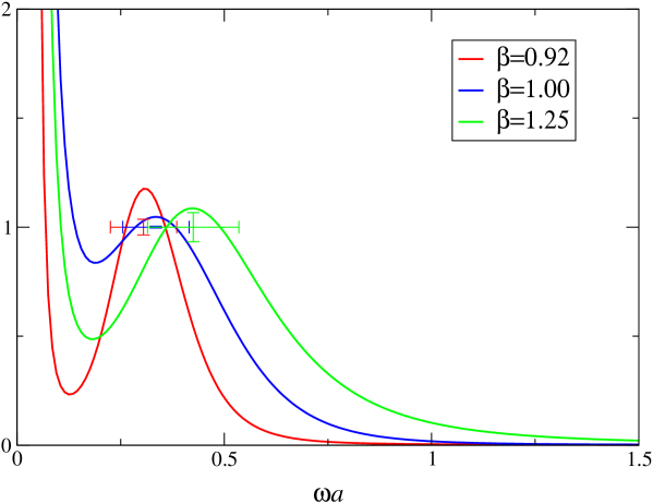
Figure 10: Rescaled Bryan image of $\rho(\omega)/\omega$ in the $\sigma$ channel from timeslices 0 – 11, for three different couplings.

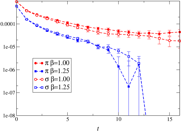
Figure 11: $\sigma$ and $\pi$ timeslice correlators from simulations of the U(1) model on a $32^{3}$ lattice.

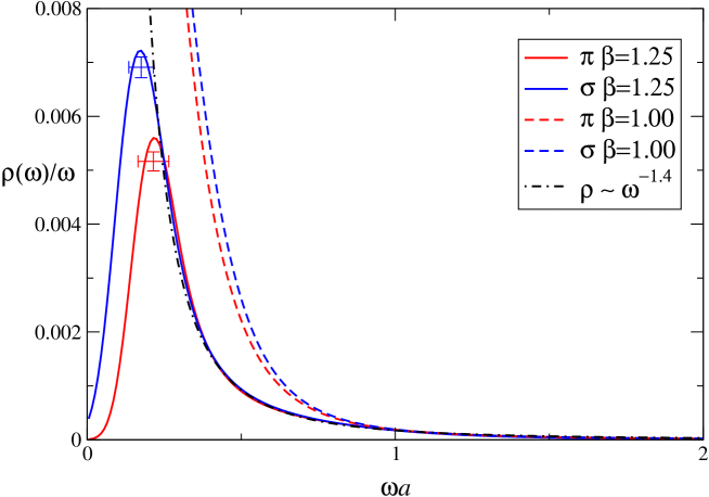
Figure 12: Bryan image of $\rho(\omega)/\omega$ in both $\sigma$ and $\pi$ channels using the correlator data of Fig. 11.

In Fig. 10 we compare the results from 3 different couplings. Since the artifact at $\omega\to 0$ distorts the normalisation of our result, we have rescaled each curve so that the rectangles of equal area to the fitted peak have the same height. The resulting curves show both the position and width of the resonance increasing with $\beta$. This is consistent with (3.3), which predicts both are proportional to a single scale $\mu$, if $\mu$ increases with $\beta$ as expected. Within errors we find the ratio of width to central position constant and approximately equal to 50%. Note, however, that ignoring the spike at $\omega=0$ the dip in the curve suggests $\lim_{\omega\to 0}\rho(\omega)/\omega\to 0$, rather than tending to a constant as predicted by (3.3).

Finally in Figs. 11 and 12 we show some results from simulations of the U(1) model. In this case it is possible to extract and compare spectra from both $\sigma$ and $\pi$ channels. The fitted time window is [1,10]. The bare fermion mass $m$ is set to zero implying that for $\beta>\beta_{c}$ the two channels should be physically indistinguishable, and Fig. 12 suggests that for large $\omega$ this is indeed the case. There is, however, a large disparity as $\omega\to 0$ between $\beta=1.00$, where $\rho(\omega)$ appears to diverge, and $\beta=1.25$ where it seems to tend smoothly to zero. Fig. 11 confirms that the behaviour of the correlators at large $t$ is not really under control yet with the precision we have been able to obtain. Also in both cases there is more power in the $\sigma$ channel at small $\omega$. This indicates we still lack a full understanding of systematics in this regime. Intriguingly, however, the large-$\omega$ behaviour is much closer to the large-$N_{f}$ prediction; the dash-dotted line in Fig. 12 is a fit of the form $\rho(\omega)\propto\omega^{-1.4}$, to be compared with the expected $\omega^{-1}$.

To summarise, there is encouraging evidence that MEM analysis can successfully identify a resonance with non-zero width in this phase of the model, whose properties are consistent, at least in part, with theoretical expectations. Despite uncertainty about the $\omega\to 0$ limit that would probably require lattices considerably longer in the Euclidean time dimension to resolve, the MEM method is capable of yielding semi-quantitative information in this regime.

5.3 The $\sigma$ Channel in the Broken Phase

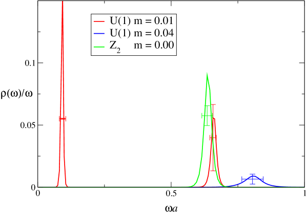
Figure 13: Rescaled Bryan image of $\rho(\omega)/\omega$ in the $\sigma$ channel from timeslices 1 – 10 at $\beta=0.65$, for two different masses in the U(1) model on a $32^{2}\times 24$ lattice, and for $m=0$ in the Z₂ model on a $24^{3}$ lattice.

Finally we return to the chirally broken phase and switch our attention to the $\sigma$ channel. Recall that since the $\sigma$ is modelled via an auxiliary boson field, diagrams formed from disconnected fermion lines are automatically included in the calculation of the correlator. The main physical issues to address are whether the the $\sigma$ is a bound state, and if it is possible to detect a signal for $\sigma\to\pi\pi$ decay. Conventional spectroscopy, using both simple pole fits and large-$N_{f}$ inspired forms which include a $f\bar{f}$-threshold, have proved at best ambiguous for this case [2]. Moreover due to the auxiliary nature of the field it is impossible to study the wavefunction, which in other channels provides clear evidence of $f\bar{f}$ binding [5].

Fig. 13 shows spectral functions in the $\sigma$ channel from simulations of the U(1) model at two different values of bare fermion mass $m$, and a comparison simulation of the massless Z₂ model, in which there is no pion degree of freedom. We used a large statistical sample; respectively $1.7\times 10^{6}$ (U(1) $ma=0.01$), $4\times 10^{5}$ (U(1) $ma=0.04$), and $1.1\times 10^{6}$ (Z₂ $m=0$) configurations were generated, and in all cases $N_{f}=4$. Since the $\sigma$ has the same quantum numbers as the vacuum, it is necessary to subtract the vacuum term $C_{vac}=\sum_{\vec{x},t}\langle\sigma(\vec{0},0)\rangle\langle\sigma(\vec{x},t)\rangle$ from the raw data to define a connected Green function. Because of statistical fluctuations this procedure is hard to implement exactly, despite the large sample generated, and we believe that uncertainity in the vacuum subtraction is the origin of the sharp spike in the U(1) $m=0.01$ spectrum centred at $\omega a=0.092$. This feature is otherwise hard to explain since the lightest particle in the spectrum (see Table 1), the $\pi$, has mass $m_{\pi}a\simeq 0.19$. We have checked that varying the subtraction constant $C_{vac}$ within a standard deviation causes dramatic alterations to both the strength and position of this feature without significantly affecting the peaks at higher $\omega$, and conclude that it is not physical.

Proceeding on this assumption we identify spectral features centred at $\omega a=0.81(2)$ (U(1) $ma=0.04$), $\omega a=0.66(1)$ (U(1) $ma=0.01$), and $\omega a=0.64(1)$ (Z₂ $ma=0$). The width of the features are $O(0.05)$ and appear stable as the number of configurations sampled is increased, which suggests they are not simple poles. Unlike the PS spectrum of Fig. 6, however, their shapes are roughly symmetric, which contrasts with the large-$N_{f}$ expectation that $\rho(\omega)$ should be sharply cut off on the low-$\omega$ side but fall away more slowly on the high-$\omega$ side due to a $f\bar{f}$ continuum. The central value of the peak for the U(1) $m=0.01$ data indicates that the state it describes is lighter than the corresponding PS state in the U(1) model (see Table 1), which has mass 0.77 – the $f\bar{f}$ threshold in this case is at 0.793(3), which lies well above the point where $\rho(\omega)/\omega$ appears to fall to zero. We deduce that for finite $N_{f}$ there is a bound state in the $\sigma$ channel, which is more tightly-bound than the PS meson for which there are no disconnected fermion line contributions. This conclusion would have been difficult to reach without MEM.

Unfortunately there is no sign of any spectral feature at the two pion threshold, expected following the discussion of Sec. 3 at $\omega a\simeq 0.38$ for $ma=0.01$ and $\omega a\simeq 0.75$ for $ma=0.04$ (implying that $\sigma\to\pi\pi$ decay is certainly possible on energetic grounds in the former case). We have checked that there is no significant difference between spectra found in U(1) and Z₂ simulations performed at the same parameter values. Possibly this is because the height of the expected feature is suppressed by a power of $1/N_{f}$ (recall (3.9)) and would need a series of simulations with varying $N_{f}$ to expose it. Thus far, however, we are unable to report observation of bound state decay in this model.

6 Summary and Outlook

Lattice simulations of theories other than quenched QCD at zero temperature will require spectrum analysis techniques of greater sophistication than the currently-used single- and multi-exponential fits, which implicitly assume a spectral density function made up from a series of isolated simple poles. In this paper we have applied one of the more promising, the Maximum Entropy Method, for the first time to a lattice model with dynamical fermions. Our main findings are summarised below:

• In the chirally broken phase of the model we have found sharply defined spectral features corresponding to the elementary fermion $f$, the simplest mesonic $f\bar{f}$ bound state, and the Goldstone boson $\pi$. These results corroborate earlier simulations [3, 5], and for the first time have permitted a plausible estimate for the meson binding energy.

• In the chirally symmetric phase we have identified a broad resonance feature whose position and width agree qualitatively with the expectations of the large-$N_{f}$ approach. The behaviour as $\omega\to\infty$ is distinct from that of an asymptotically-free theory, and is evidence for a non-perturbative anomalous dimension associated with a UV renormalisation group fixed point.

• In the chirally broken phase we have made the first quantitative study of the $\sigma$ channel, and found that it is more tightly bound than the conventional PS meson, possibly due to the additional contribution of disconnected fermion line diagrams. We have been unable to find evidence for $\sigma\to\pi\pi$ decay.

Since the philosophy of the MEM method is to make the maximum possible use of data, we have used correlator data from as wide a time window as possible consistent with stability of the fit. The main problem we have faced has been systematic errors associated with the upper end of the time window used in the fit, particularly since we have been anxious to avoid finite volume effects. This has made it impossible to have control of the $\omega\to 0$ limit. As explained in Sec. 5.3, in the $\sigma$ channel there may also be artifacts associated with vacuum subtraction. Overall, our conclusion is that MEM has proved a useful semi-quantitative analysis tool, but that there remains room for improvement.

In the future it will be interesting to study 2+1$d$ four-fermion models at non-zero temperature and/or density. Since spectral analysis requires data from many Euclidean time separations to be effective, it is likely to be some time before an equivalent analysis can be applied to QCD with dynamical fermions. However, in the vicinity of the deconfining/chiral symmetry restoring transition the dominant modification to the zero-$T$ spectrum is expected to be collision-broadening due to pions, an effect absent from quenched QCD, where the lightest states are glueballs, but in principle present in the current model. Additionally, there is no longer any ambiguity about the IR cutoff, which is now $T^{-1}$, and the $\omega\to 0$ limit should become accessible [10]; the slope of $\rho(\omega)$ in this limit yields information about transport coefficients such as electrical conductivity via the Kubo formula [18]. Finally, the four-fermi model is currently the only model simulable at non-zero baryon chemical potential $\mu$ which has a Fermi surface [4]; there may be rich physics associated with phenomena such as first and zero sound or superfluidity via BCS condensation to explore.

References

- [1] B. Rosenstein, B.J. Warr and S.H. Park, Phys. Rep. 205, 59 (1991).
- [2] S.J. Hands, A. Kocić and J.B. Kogut, Ann. Phys. 224, 29 (1993).
-
[3]
S.J. Hands, S. Kim and J.B. Kogut, Nucl. Phys. B442, 364 (1995);
I.M. Barbour, S.J. Hands, J.B. Kogut, M.-P. Lombardo and S.E. Morrison, Nucl. Phys. B557, 327 (1999). -
[4]
K.G. Klimenko, Z. Phys. C37, 457 (1988);
B. Rosenstein, B.J. Warr and S.H. Park, Phys. Rev. D39, 3088 (1989);
S.J. Hands, A. Kocić and J.B. Kogut, Nucl. Phys. B390, 355 (1993);
R. Gatto, M. Modugno and G. Pettini, Phys. Rev. D57, 4995 (1998);
J.B. Kogut, M.A. Stephanov and C.G. Strouthos, Phys. Rev. D58:096001 (1998);
J.B. Kogut and C.G. Strouthos, Phys. Rev. D63:054502 (2001);
E. Babaev, Phys. Lett. B497, 323 (2001);
S.J. Hands, J.B. Kogut and C.G. Strouthos, Phys. Lett. B515, 407 (2001);
S.J. Hands, B. Lucini and S.E. Morrison, Phys. Rev. D65:036004 (2002). - [5] S.J. Hands, J.B. Kogut and C.G. Strouthos, Phys. Rev. D65:114507 (2002).
- [6] E.V. Shuryak, Rev. Mod. Phys. 65, 1 (1993).
-
[7]
M.C. Chu, J.M. Grandy, S. Huang and J.W. Negele, Phys. Rev.
D48, 3340 (1993);
D.B. Leinweber, Phys. Rev. D51, 6369 (1995);
S.J. Hands, P.W. Stephenson and A. McKerrell, Phys. Rev. D51, 6394 (1995);
A. Bochkarev and P. de Forcrand, Nucl. Phys. B477, 489 (1996);
C.R. Allton and S. Capitani, Nucl. Phys. B526, 463 (1998). - [8] M. Asakawa, Y. Nakahara and T. Hatsuda, Prog. Part. Nucl. Phys. 46, 459 (2001).
-
[9]
M. Asakawa, Y. Nakahara and T. Hatsuda, Phys. Rev. D60:091503, (1999);
M. Oevers, C.T.H. Davies and J. Shigemitsu, Nucl. Phys. Proc. Suppl. 94, 423 (2001);
I. Wetzorke and F. Karsch, in Strong and Electroweak Matter 2000, ed. C.P. Korthals-Altes (World Scientific 2001) p. 193, hep-lat/0008008;
J. Clowser and C.G. Strouthos, Nucl. Phys. Proc. Suppl. 106, 489 (2002) - [10] F. Karsch, E. Laermann, P. Petreczky, S. Stickan and I Wetzorke, Phys. Lett. B530, 147 (2002).
- [11] H. Jeffreys, Theory of Probability, 3rd edition (Oxford Univ. Press, Oxford, 1998).
- [12] S. Brandt, Statistical and Computational Methods in Data Analysis. (North-Holland, 1983).
-
[13]
J. Skilling,
in Maximum Entropy and Bayesian Methods, p. 45
(Kluwer Academic, London, 1989);
S.F. Gull, ibid. p. 53.;
E.T. Jaynes, in Maximum Entropy and Bayesian Methods in Applied Statistics, p. 26 (Cambridge University Press, Cambridge, 1986);
J. Skilling, in Maximum Entropy and Bayesian Methods in Science and Engineering, Vol 1, p. 173. (Kluwer Academic, London, 1988). - [14] R.K. Bryan, Eur. Biophys. J. 18, 165 (1990).
- [15] Y. Kikukawa and K. Yamawaki, Phys. Lett. B234, 497 (1990).
- [16] M. Abramowitz and I.A. Stegun, Handbook of Mathematical Functions, ch. 5 (Dover, New York, 1972).
- [17] R. Gupta, G. Guralnik, G.W. Kilcup and S.R. Sharpe, Phys. Rev. D43, 2003 (1991).
-
[18]
J.M. Martinez Resco and M.A. Valle Basagoiti, Phys. Rev.
D63:056008 (2001);
G. Aarts and J.M. Martinez Resco, JHEP 0204:053 (2002).