One-loop matching coefficients for improved staggered bilinears

Abstract

We calculate one-loop matching factors for bilinear operators composed of improved staggered fermions. We compare the results for different improvement schemes used in the recent literature, all of which involve the use of smeared links. These schemes aim to reduce, though not completely eliminate, $O(a^{2})$ discretization errors. We find that all these improvement schemes substantially reduce the size of matching factors compared to unimproved staggered fermions. The resulting corrections are comparable to, or smaller than, those found with Wilson and domain-wall fermions. In the best case (“Fat-7” and mean-field improved HYP links) the corrections are $10\%$ or smaller at $1/a=2\;$GeV.

I Introduction

Improved staggered fermions are an attractive choice for numerical simulations of unquenched QCD [1, 2, 3, 4, 5, 6, 7, 8, 9, 10, 11]. They maintain the positive features of unimproved staggered fermions—smaller CPU requirements than other fermion discretizations, a remnant chiral symmetry, and $O(a^{2})$ discretization errors—while potentially avoiding its drawbacks—large flavor symmetry breaking and large perturbative matching factors. We have begun a program of calculations of electroweak matrix elements using these fermions, and thus need to decide between the different improvement schemes that have been suggested in the recent literature. Since we intend at first to use one-loop perturbation theory to match lattice and continuum operators, it is important that the matching factors for relevant operators are close to unity. In this paper we calculate these matching factors for the bilinear operators which form the building blocks of the four-fermion operators we intend to use in our matrix element calculations. We expect our results to be a good guide to the size of corrections for the four-fermion operators themselves—typically the one-loop contributions get roughly doubled. In any case, finding small one-loop corrections for bilinears is a prerequisite for proceeding to four-fermion operators.

We stress that we are using the term “improvement” loosely in this work. Although the improved actions and operators that we use are motivated by the Symanzik program, we are not following this program systematically. This would involve improving the gauge and fermion actions, and the operators, so as to remove $O(a^{2})$ errors either order by order in perturbation theory or non-perturbatively. Such a program is much more difficult for staggered fermions than for Wilson-like fermions, particularly with the operators we use which are spread out over a $2^{4}$ hypercube. Our aim is to change the fermion action and operators such that the $O(a^{2})$ corrections are reduced from the large size typical of unimproved staggered fermions to the size seen with Wilson, Domain wall or overlap fermions. We do not improve the gauge action.

The plan of this paper is as follows. In the next section we describe the alternatives we have considered for improved operators and actions. Section III collects the new features of the Feynman rules that are introduced by improvement. In sec. IV we present analytic results for the one-loop matching constants. We then, in sec. V, describe how to do a second level of mean-field improvement of the bilinear operators. We close in sec. VI with the numerical results and a discussion of their implications. We collect some definitions in an Appendix, along with the results that allow us to push the analytic calculation one step further than in previous work.

We lean heavily on the notation and methodology of Ref. [14], and for brevity we refer to that paper as PS in the following.

II Improved actions and operators

Lepage [2, 8] and Lagae and Sinclair [6] have argued that flavor symmetry breaking can be substantially reduced by suppressing the coupling of high momentum gluons which connect “physical” quarks residing at different corners of the Brillouin zone. Such suppression is also expected to reduce the size of one-loop contributions to perturbative matching factors, since, as noted by Golterman [15], their size is largely due to tadpole-type diagrams which involve these flavor-changing vertices.

The flavor-changing coupling can be suppressed by replacing the standard “thin” link with some form of “smeared” link in the quark covariant derivative. Various options have been tried, and we consider here two choices which have been successful at reducing flavor symmetry breaking in pion masses, are relatively local, and have been extensively studied: the “Fat-7” link introduced by Orginos and Toussaint [7] and studied numerically by the MILC collaboration [10], and the HYP link introduced by Hasenfratz and Knechtli [16]. We refer to the original papers for the details of the constructions and do not repeat them here. Both are “fattened” by averaging over paths containing links in some or all of the transverse directions (and which in the Fat-7 case are up to 7 links long), and in this way they reduce the coupling to gluons with transverse momenta of $O(1/a)$. In some sense the Fat-7 link is the simplest choice which accomplishes this, while the HYP link involves an average over more paths. On the other hand, the HYP link involves three levels of APE-like smearing with projection back into SU(3). Simulations show that such smearing is very effective at reducing flavor-symmetry breaking. Indeed, using the HYP links leads to a greater reduction in flavor symmetry breaking than the Fat-7 links.

The introduction of smeared links can be viewed as one part of the Symanzik improvement program applied at tree-level to staggered fermions. Complete removal of $O(a^{2})$ terms from fermion vertices requires two other improvements [8]. First, the smearing of the links introduces an $O(a^{2})$ correction to the flavor-conserving quark-gluon coupling. This can be removed by a adding to the smearing a 5-link “double staple”—we refer to this as the “Lepage term”. Second, the $O(a^{2})$ corrections to the fermion propagator need to be removed, and this can be done by adding a next-to-nearest-neighbor derivative, the “Naik term” [19].

An observation of practical relevance is that the Naik term is the only part of the improvement of the fermion vertex that cannot be accomplished simply by changing the links in the unimproved staggered action. In other words, if one does not include the Naik term, and if one is interested in calculating propagators on configurations that have been already been generated (whether quenched or unquenched) then the practical implementation of smeared links is simple: one calculates the smeared links, and then uses an unimproved staggered inverter.

Complete tree-level $O(a^{2})$ improvement of physical quantities requires, in addition to the improvement of fermion vertex outlined above, the use of a tree-level (or more highly) improved gauge action. The previous discussion implies, however, that $O(a^{2})$ errors from the gauge action are not responsible for the large flavor-symmetry breaking or the large “tadpole” contributions to matching factors.

With these general comments in mind, we can now explain our choices of action and operators. We use the single-plaquette Wilson gauge action, since this is the action we are using in our present simulations. For the fermion action, we keep the original staggered form (without the Naik term), but use various types of smeared links. The only exception is case (5) below, in which we keep the Naik term. Finally, for the bilinears we use the standard hypercube form (the definition of which is given in the Appendix), rendered gauge invariant by including the average of the product of links along the shortest paths between the quark and anti-quark field. The only improvement of the operators that we consider is the use of smeared links. Intuitively, the reduction in fluctuations in these links will reduce the flavor symmetry breaking between bilinears [16]. In all cases we use the same type of smeared links in the operators as in the action, so that the hypercube vector current is conserved [except in case (5)].

The specific choices of links we consider are:

1. The original gauge links, tadpole improved (following the prescription of Ref. [18] as implemented in PS). We use the fourth root of the average plaquette to determine the “average link” $u_{0}$. This yields (tadpole-improved) unimproved staggered fermions and unimproved operators, and allows us to check our results against those in PS.

2. Fat-7 smeared links, built out of tadpole improved links (as in the numerical implementation of Ref. [7, 10]). We stress again that we use these smeared links both in the action and in the bilinear operators.

3. Fully $O(a^{2})$ improved smeared links, i.e. Fat-7 links with the Lepage “double-staple” term added, again both in the action and the operators.

4. Links smeared according the HYP prescription of Hasenfratz and Knechtli [16], again both in the action and the operators. Three parameters, $\alpha_{1-3}$, need to be specified to completely define HYP smearing, and we focus on two choices, as described below. We also consider a variant in which we tadpole improve the smeared links themselves (section V).

In addition, we consider a final choice of action and operators:

1. Following the “Asqtad” action introduced by Lepage [8] and used extensively by the MILC collaboration [10], we add the Naik term to the action of choice 3, while taking the same operators as in choice 3. In the Naik term alone, we use the original unsmeared gauge links (tadpole improved).

This differs from the “Asqtad” action, however, because we use the unimproved Wilson gauge action, whereas “Asqtad” includes an improved gauge action. We thus refer to our choice as the “Asqtad-like” action. Our expectation is that the choice of gauge action has relatively little impact on the size of matching factors, and particularly on the variation of these factors between bilinears having the same spin and different flavor.

III Feynman rules

The Feynman rules for unimproved staggered fermions are standard. In the notation we use here, they can be found in PS, and we do not repeat them. We discuss only the changes introduced by smearing the links and including the Naik term.

We consider first the effect of smearing the links. For all except tadpole diagrams (i.e. those in which two gluons emerge from a single, possibly smeared, link), the only effect is to change the coupling to the underlying gluon field. With the unimproved action, a link in the $\mu$-th direction couples only to a gluon $A_{\nu}(k)$ with $\nu=\mu$. The smeared links, however, couple to $A_{\nu}(k)$ for all $\nu$, and the extra factor this introduces can be conveniently written as

$$\delta_{\nu,\mu}D_{\mu}(k)+(1-\delta_{\nu,\mu})G_{\nu,\mu}(k)\,.$$ (1)

The diagonal and off-diagonal couplings can be decomposed, respectively, as

$$D_{\mu}(k)=1-d_{1}\sum_{\nu\neq\mu}{\bar{s}}_{\nu}^{2}+d_{2}\sum_{\nu<\rho\atop\nu,\rho\neq\mu}{\bar{s}}_{\nu}^{2}{\bar{s}}_{\rho}^{2}-d_{3}{\bar{s}}_{\nu}^{2}{\bar{s}}_{\rho}^{2}{\bar{s}}_{\sigma}^{2}-d_{4}\sum_{\nu\neq\mu}{\bar{s}}_{\nu}^{4}\,,$$ (2)

with ${\bar{s}}_{\nu}=\sin(k_{\nu}/2)$, etc., and

$$G_{\nu,\mu}(k) = {\bar{s}}_{\mu}{\bar{s}}_{\nu}\widetilde{G}_{\nu,\mu}(k)$$ (3)

$$\widetilde{G}_{\nu,\mu}(k) = d_{1}-d_{2}\frac{({\bar{s}}_{\rho}^{2}+{\bar{s}}_{\sigma}^{2})}{2}+d_{3}\frac{{\bar{s}}_{\rho}^{2}{\bar{s}}_{\sigma}^{2}}{3}+d_{4}{\bar{s}}_{\nu}^{2}\,,$$ (4)

where all indices ($\mu,\nu,\rho,\sigma$) are different.

The coefficients $d_{1-4}$ distinguish the different choices of links:

1. Unimproved (choice 1 above):

   $$d_{1}=0,\quad d_{2}=0,\quad d_{3}=0,\quad d_{4}=0.$$ (5)

2. Fat-7 links (choice 2 above):

   $$d_{1}=1,\quad d_{2}=1,\quad d_{3}=1,\quad d_{4}=0.$$ (6)

3. $O(a^{2})$ improved links (choices 3 and 5 above):

   $$d_{1}=0,\quad d_{2}=1,\quad d_{3}=1,\quad d_{4}=1.$$ (7)

4. HYP smeared links (choice 4 above):

   $$d_{1}=(2/3)\alpha_{1}(1+\alpha_{2}(1+\alpha_{3})),\quad d_{2}=(4/3)\alpha_{1}\alpha_{2}(1+2\alpha_{3}),\quad d_{3}=8\alpha_{1}\alpha_{2}\alpha_{3},\quad d_{4}=0.$$ (8)

   We consider two choices for the $\alpha_{i}$. The first was determined in Ref. [16] using a non-perturbative optimization procedure: $\alpha_{1}=0.75$, $\alpha_{2}=0.6$ $\alpha_{3}=0.3$. This gives

   $$d_{1}=0.89\,,\quad d_{2}=0.96\,,\quad d_{3}=1.08\,,\quad d_{4}=0\,.$$ (9)

   The second is chosen so to remove $O(a^{2})$ flavor-symmetry breaking couplings at tree level. This choice, $\alpha_{1}=7/8$, $\alpha_{2}=4/7$ and $\alpha_{3}=1/4$, gives

   $$d_{1}=1,\quad d_{2}=1,\quad d_{3}=1,\quad d_{4}=0,$$ (10)

   i.e. the same as for Fat-7 links.

These results agree with those of Refs. [20, 21], but are written here in a somewhat different notation. The fact that all four choices can be collected in this form simplifies the resulting one-loop calculations. It is particularly noteworthy that the Fat-7 and HYP vertices can be made identical, showing that these two choices cannot be distinguished by their flavor breaking effects in perturbation theory [21]. The one-loop matching factors for these two choices are not, however, identical, because the tadpole contributions differ.

For tadpole diagrams, which involve two-gluon vertices, the differences between the actions are more complicated, and will be given explicitly below.

The inclusion of the Naik term alters the Feynman rules in several ways. In the fermion propagator, all factors of $s_{\mu}=\sin p_{\mu}$ are replaced:

$$s_{\mu}\longrightarrow s^{N}_{\mu}=s_{\mu}(1+d_{N}s_{\mu}^{2}/6)\,.$$ (11)

Here we have introduced a fifth coefficient $d_{N}$ which distinguishes the different choices of action: $d_{N}=0$ unless the Naik term is included, in which case $d_{N}=1$. This device allows us to write most of our results in a way which holds for all choices of action and operators.

The one-gluon vertex is also changed by the Naik term, but this can only be represented in a simple way if one of the quarks in the vertex has vanishing physical momentum [$k_{\mu}=(0,\pi/a)$]. In this case, the diagonal part of the vertex changes as follows:

$$D_{\mu}\rightarrow D^{N}_{\mu}=D_{\mu}+d_{N}s_{\mu}^{2}/6\,.$$ (12)

This substitution works for all except the self-energy diagram, which we consider explicitly below.

IV Analytic results for matching constants

The one-loop matching relations take the general form,

$${\cal O}_{i}^{{\rm cont}}={\cal O}_{i}^{{\rm lat}}+C_{F}{g^{2}\over 16\pi^{2}}\sum_{j}(\delta_{ij}2d_{i}\ln(\mu a)+c_{ij}){\cal O}_{j}^{{\rm lat}}$$ (13)

where $C_{F}=4/3$ is the color Casimir factor, $\mu$ is the renormalization scale of the continuum operators, and $i$ and $j$ run over all the different possible bilinears in a four-flavor theory. The explicit forms of the operators are given in the Appendix. The constants $d_{i}$ are proportional to the one-loop anomalous dimensions of the bilinears, $\gamma_{i}^{(0)}=-2C_{F}d_{i}$. They depend only on the spin of the bilinear, and are $d_{i}=(3,0,-1)$ for spins $(S/P,V/A,T)$. The finite part of the coefficient can be written

$$c_{ij}=\delta_{ij}\left[d_{i}(\gamma_{E}-F_{0000})+t_{S}\right]-c^{1}_{ij}\,,$$ (14)

with $t_{S}$ depending on the continuum renormalization scheme. For the NDR scheme $t_{S}=(-0.5,0,1.5)$ for spins $(S/P,V/A,T)$. The conversion to other schemes is given in PS. The constants are $\gamma_{E}=0.577216$ and $F_{0000}=4.36923$. Finally, the “lattice” part of the coefficient can be broken up as follows:

$$c^{1}_{ij}=X_{ij}+\delta_{ij}\left(Y_{i}+T_{i}+Z\right)\,.$$ (15)

Here $X$, $Y$, $T$ and $Z$ refer to contributions from the different types of diagrams using the notation of PS, as illustrated in Fig. 1. This equation incorporates the fact, derived below, that only the $X$ diagrams lead to mixing among bilinears.

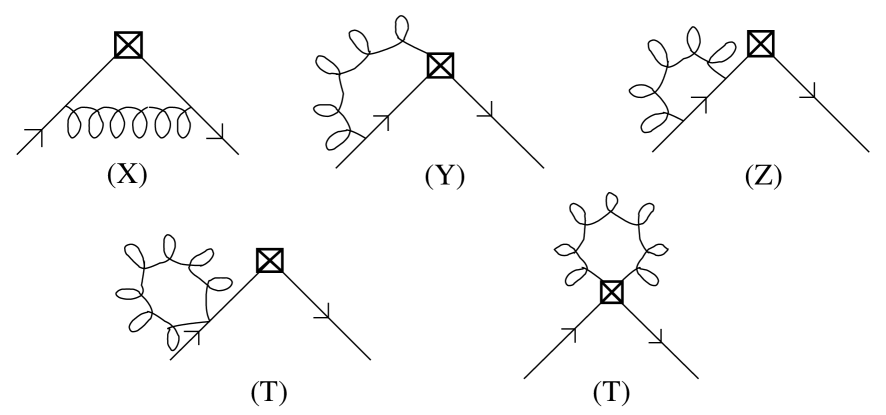
FIG. 1.: Notation for diagrams contributing to matching factors.

All our calculations are done in Feynman gauge. We have checked our results by doing two independent calculations using different methods—the first following PS and the second using the methods presented in Refs. [22, 23].

A $X$ diagrams

The calculation follows the same steps as in PS, except for two changes.

• We have been able to carry out the calculation analytically apart from one final integral, using the results (A8,A9) given in the Appendix.

• The improved vertex eq. (1) allows propagation from a smeared link in the $\mu$-th direction to another in any direction, even in Feynman gauge. It is useful to distinguish between the case where the second link is also in the $\mu$-th direction, for which the gluon propagator is multiplied by

  $$P^{NN}_{\mu}(k)=D^{N}_{\mu}(k)^{2}+\sum_{\nu\neq\mu}G_{\nu,\mu}(k)^{2}\,,$$ (16)

  and the case where the second link is in a different direction $\rho\neq\mu$, for which the multiplying factor is

  $$D^{N}_{\mu}G_{\mu,\rho}+D^{N}_{\rho}G_{\rho,\mu}+\sum_{\nu\neq(\mu,\rho)}G_{\nu,\mu}G_{\nu,\rho}\equiv\ 4\bar{s}_{\mu}\bar{s}_{\rho}O^{NN}_{\mu\rho}(k)\,.$$ (17)

  The superscripts emphasize the fact that there is a possible Naik term at both ends of the propagator.

Using these results, we find the following expression for the diagonal part of the contributions from the $X$ diagrams:

$$X_{ii} = \sum_{\mu,\rho}\int_{k}\left[\bar{c}_{\mu}^{2}P^{NN}_{\mu}(s^{N}_{\rho})^{2}BF^{2}V_{i}(k)-\frac{B^{2}}{4}\right](-1)^{\widetilde{S}_{\mu}+\widetilde{S}_{\rho}}$$ (19)

$$\mbox{}+2\sum_{\mu<\nu}\int_{k}s_{\mu}s^{N}_{\mu}s_{\nu}s^{N}_{\nu}O^{NN}_{\mu\nu}BF^{2}V_{i}(k)\left[1-(-1)^{\widetilde{S}_{\mu}+\widetilde{S}_{\nu}}\right]\,.$$

Here $\int_{k}\equiv 16\pi^{2}\prod_{\mu}\int_{-\pi}^{\pi}{dk_{\mu}\over 2\pi}$, $\bar{c}_{\mu}=\cos(k_{\mu}/2)$ and $s_{\mu}=\sin(k_{\mu})$. The functions arising from boson and fermion propagators are, respectively,

$$B(k)={1\over 4\sum_{\mu}\bar{s}_{\mu}^{2}}\,,\qquad F(k)={1\over\sum_{\mu}(s^{N}_{\mu})^{2}}\,.$$ (20)

For the sake of brevity we do not show the argument $k$ of these functions or of $P^{NN}_{\mu}$ and $O^{NN}_{\mu\nu}$ in eq. (19) and in the following. The index $i$ in eq. (19) labels the spin and flavor of the operator, and the $B^{2}/4$ term on the first line is the conventional integral used to cancel divergences. The function $V_{i}(k)$ is defined in eq. (A8); we stress again that the use of this equation leads to a simpler form than that given in PS.

Only the $X$ diagrams lead to mixing, i.e. non-zero values for $X_{ij}$, $i\neq j$. We find that we can also give explicit expressions for the mixing terms using eq. (A9). As for unimproved staggered fermions, the mixing that occurs at one-loop turns out to be only a subset of that allowed by the hypercubic symmetry group. The non-zero mixing coefficients are (using the definitions in PS—see table II)

$$c_{VVM} = \int_{k}4BF^{2}s_{1}s^{N}_{1}s_{2}s^{N}_{2}(P^{NN}_{3}\bar{c}_{3}^{2}-O^{NN}_{12}s_{3}^{2})\,,$$ (21)

$$c_{VAM} = \int_{k}4BF^{2}s_{1}s^{N}_{1}s_{2}s^{N}_{2}(-P^{NN}_{3}\bar{c}_{3}^{2}c_{3}c_{4}+O^{NN}_{12}s_{3}^{2}[2c_{2}-c_{3}]c_{4})\,,$$ (22)

$$c_{VTM} = \int_{k}2BF^{2}s_{1}s^{N}_{1}s_{2}s^{N}_{2}(-P^{NN}_{3}\bar{c}_{3}^{2}[c_{3}+c_{4}]+O^{NN}_{12}s_{3}^{2}[2c_{2}-c_{3}+c_{4}])\,,$$ (23)

$$c_{TAM} = \int_{k}2BF^{2}s_{1}s^{N}_{1}s_{2}s^{N}_{2}(P^{NN}_{3}\bar{c}_{3}^{2}[c_{4}-c_{3}]+O^{NN}_{12}s_{3}^{2}[2c_{2}-c_{3}-c_{4}])\,,$$ (24)

where $c_{\mu}=\cos(k_{\mu})$.

B $Y$ diagrams

$Y$ diagrams involve the gluon connecting an external quark or antiquark line to the operator. As explained in PS, with the unimproved staggered action and unsmeared links, $Y$ diagrams do not lead to mixing between different bilinears, and the result depends only on the “distance”, $\Delta=\sum_{\mu}(S-F)_{\mu}^{2}$, of the bilinear. It is straightforward, though tedious, to check that these arguments generalize to the improved actions considered here. The result is

$$Y_{\Delta}=Y_{\Delta-1}+I_{\Delta}\qquad(\Delta>0)\,,$$ (25)

with $Y_{\Delta=0}=0$, and

$$I_{\Delta} = \int_{k}BFs_{1}s^{N}_{1}P^{N}_{1}V_{Y}(\Delta)+\int_{k}12BF\bar{s}_{1}^{2}s_{2}s^{N}_{2}O^{N}_{21}V_{Y}(\Delta)$$ (26)

$$V_{Y}(1) = 1\,,\ \ V_{Y}(2)=\frac{c_{2}+c_{3}+c_{4}}{3}\,,\ \ V_{Y}(3)=\frac{c_{2}c_{3}+c_{2}c_{4}+c_{3}c_{4}}{3}\,,\ \ V_{Y}(4)=c_{2}c_{3}c_{4}\,.$$ (27)

The new functions are defined by

$$P^{N}_{\mu}(k)\equiv D^{N}_{\mu}(k)D_{\mu}(k)+\sum_{\nu\neq\mu}G_{\nu,\mu}(k)^{2}\,,$$ (28)

and

$$4\bar{s}_{\mu}\bar{s}_{\rho}O^{N}_{\mu\rho}(k)\ \equiv\ D^{N}_{\mu}G_{\mu,\rho}+D_{\rho}G_{\rho,\mu}+\sum_{\nu\neq(\mu,\rho)}G_{\nu,\mu}G_{\nu,\rho}\,.$$ (29)

The single superscript “$N$” reflects the fact that the Naik term appears only at the quark-gluon vertex and not in the operator. Note that, unlike $O^{NN}_{\mu\rho}$, $O^{N}_{\mu\rho}$ is not symmetrical.

C Tadpole diagrams

Here we include tadpole diagrams both on the external quark and antiquark propagators (i.e. self-energy contributions), and those coming from the bilinear. In the latter case we include all diagrams in which the two gluons both come from the bilinear, irrespective of whether they emanate from the same smeared link. Thus, for the example of a distance-2 bilinear, which involves an average of a sum of products of two links, the gluon can couple between the links (as well as going from each link back to itself).

It is convenient to divide the contribution into two parts,

$$T_{i}=T_{i}^{a}+T_{i}^{b}\,,$$ (30)

with the former coming from gluon loops beginning and ending on the same smeared link, and the latter involving gluons propagating between smeared links. In both cases the result depends only on the distance $\Delta$ of the bilinear.

No simple general formula covers all choices of links and action, so we quote the results in turn.

1. For unimproved staggered fermions, the result is (PS)

   $$T^{a}_{\Delta}=(\Delta-1)\left(\pi^{2}-\int_{k}B/2\right)\,,$$ (31)

   where the factor of $\pi^{2}$ comes from tadpole improvement using the fourth-root of the plaquette. If one uses the trace of the Landau gauge link, then $\pi^{2}$ is replaced by $\int_{k}3B/8$.

2. For the Fat-7 links (without the Naik term), the result is the same as for unimproved staggered fermions, eq. (31), due to cancellations.

3. For $O(a^{2})$ improved links (but without the Naik term), we find

   $$T^{a}_{\Delta}=(\Delta-1)\left[\left(\pi^{2}-\int_{k}B/2\right)+{3\over 2}\int_{k}Bc_{1}\bar{s}_{2}^{2}\right]\,.$$ (32)

4. For HYP links, we find

   $$T^{a}_{\Delta}=(\Delta-1)\int_{k}(-B/2)P_{1}\,,$$ (33)

   where $P_{\mu}$ contains no Naik vertices:

   $$P_{\mu}(k)=D_{\mu}(k)^{2}+\sum_{\nu\neq\mu}G_{\nu,\mu}(k)^{2}\,.$$ (34)

   We emphasize that, at this stage, there is no tadpole improvement factor for the HYP links (although a related mean-field improvement will be introduced in sec. V). It is also noteworthy that this result would apply for both the Fat-7 and $O(a^{2})$ improved links were one to also include projection back into SU(3) in those cases [24].

5. Finally, for the Asqtad-like action we find

   $$T^{a}_{\Delta}=(\Delta-1)\left[\left(\pi^{2}-\int_{k}B/2\right)+{3\over 2}\int_{k}Bc_{1}\bar{s}_{2}^{2}\right]+{1\over 4}\left[\pi^{2}-\int_{k}Bc_{1}(1+c_{1})\right]\,,$$ (35)

   in which the second contribution is due to the Naik term.

Now we turn to the “off-diagonal” tadpoles. These only arise from the bilinears, and not from the self-energy contributions, and are only present for operators with $\Delta\geq 2$. Since they are off-diagonal they are not affected by $SU(3)$ projection, and so take a common form for all actions and operators:

$$T_{\Delta}^{b} = 4\int_{k}B\bar{s}_{1}^{2}\bar{s}_{2}^{2}O_{12}V_{T}(\Delta)$$ (36)

$$V_{T}(2) = 1\,,\ \ V_{T}(3)=2+c_{3}\,,\ \ V_{T}(3)=3+2c_{3}+c_{3}c_{4}\,.$$ (37)

Here $O_{12}$ does not contain Naik contributions, even for the Asqtad-like action:

$$4\bar{s}_{\mu}\bar{s}_{\rho}O_{\mu\rho}(k)\ \equiv\ D_{\mu}G_{\mu,\rho}+D_{\rho}G_{\rho,\mu}+\sum_{\nu\neq(\mu,\rho)}G_{\nu,\mu}G_{\nu,\rho}\,.$$ (38)

D Self-energy diagrams

If the Naik term is not included in the action, the flavor-singlet vector current is conserved, and it follows from the corresponding Ward Identity that its matching factor vanishes. Thus it must be that, in cases 1-4,

$$Z=-X_{ii}-Y_{1}\,,\qquad i=(\gamma_{\mu}\otimes 1)\,.$$ (39)

Here we have used the result that $T_{1}=0$ for cases 1-4. We have checked eq. (39) analytically and numerically.

We cannot use this relation for the Asqtad-like action, since the hypercube vector operator is not the conserved current (as it does not contain a Naik-like contribution). A direct calculation is needed, and we find:

$$Z = \int_{k}B^{2}+\int_{k}BFI_{Z}\,,$$ (40)

$$I_{Z} = c_{1}(1+d_{N}s_{1}^{2}/2)(1-2(s_{1}^{N})^{2}F)\left(\bar{c}_{1}^{2}P_{1}^{NN}-3\bar{c}_{2}^{2}P_{2}^{NN}\right)$$ (44)

$$\mbox{}-s_{1}s_{1}^{N}\left(P_{1}+d_{N}(2s_{1}^{2}/3-\bar{c}_{1}^{2})D_{1}-d_{N}s_{1}^{2}\bar{c}_{1}^{2}c_{1}/6\right)$$

$$\mbox{}-12s_{1}s_{1}^{N}c_{1}(1+d_{N}s_{1}^{2}/2)s_{2}s_{2}^{N}FO_{12}^{NN}$$

$$\mbox{}-3\bar{s}_{1}^{2}s_{2}s_{2}^{N}\left(4O_{12}-d_{N}c_{1}\bar{c}_{1}^{2}\widetilde{G}_{1,2}+d_{N}s_{2}^{2}\widetilde{G}_{2,1}/6\right)\,.$$

The first term in $Z$ is the standard integral used to subtract the divergent piece. We have inserted $d_{N}$ in appropriate places so that this result is valid for all the actions we consider.

V Further mean-field improvement of operators

It is possible to apply another level of tadpole, or, more accurately, mean-field, improvement to the operators and actions which involve smeared links. Actually, for the HYP smeared links, this is the first level of tadpole improvement. The fluctuations in the smeared links are reduced compared to those of the original links but are still present. The residual fluctuations can be estimated and partially removed by defining a smeared mean-link by analogy with the definition of the original mean-link [18]:

$$(u_{0}^{SM})^{4}=\langle\mathrm{Smeared-Plaquette}\rangle\,.$$ (45)

Here the “smeared-plaquette” means the plaquette built out of smeared links. The operators are then mean-field improved by multiplying them by

$$(u_{0}^{SM})^{1-\Delta}\,,$$ (46)

where $\Delta$ is the number of links in the bilinear. The argument leading to this factor is identical to that used in PS when tadpole improving staggered operators, and we do not repeat it here. This procedure should be simple to implement in practice.

We have calculated the effect of such a mean-field improvement for Fat-7, $O(a^{2})$ improved, and HYP links. We have not applied it to the case of the Asqtad-like action, because it is not entirely clear to us how to incorporate the Naik term. We find that one must add to the tadpole contribution the following:

$$T_{\Delta}^{c}=(\Delta-1)\left[-T^{a}_{\Delta=2}-T^{b}_{\Delta=2}-\int_{k}BP_{1}c_{2}/2\right]\,,$$ (47)

where $T^{a,b}_{\Delta}$ and $P_{1}$ are given in the previous section. The quantity in square parentheses evaluates to $-0.9125$ for Fat-7 links, $-4.0634$ for $O(a^{2})$ improved links, $0.5782$ for HYP links with $\alpha_{1-3}=0.75,0.6,0.3$, and to $1.0538$ for HYP links with the “Fat-7 choice” $\alpha_{1-3}=7/8,4/7,1/4$. These values are substantially smaller than the analogous factor in the tadpole improvement of the unsmeared links, namely $\pi^{2}$. They are, nevertheless, significant, as we see in the next section.

It is noteworthy that the Fat-7 and $O(a^{2})$ improved smeared links receive a mean-field correction of opposite sign to that of both the HYP links. This indicates that the fluctuations in the former case have been “overcompensated” by smearing, and suggests that this higher level of mean-field improvement is likely to be more significant for the HYP smeared links.

Finally, we note that after this higher level of mean-field improvement, the results for Fat-7 and HYP links with $\alpha_{1-3}=7/8,4/7,1/4$ are identical. The equality of the tadpole contributions can be seen by combining eqs. (31), (33) and (47); that of other contributions follows from the fact that the single-gluon vertex is the same in both cases.

VI Numerical results and discussion

We present numerical results for the matching coefficients in Tables I–III. As explained in Ref. [17], the corrections are unchanged if the operators are multiplied by $(\gamma_{5}\otimes\xi_{5})$, due to the conserved axial symmetry. Thus we show results for only half the operators. Recall that we have chosen the NDR scheme ($\overline{MS}$ with an anticommuting $\gamma_{5}$) and set $\mu=1/a$. We expect this to be a reasonable choice for the matching scale, but, in any case, the dependence of the $c_{ij}$ on $\mu$ is weak, as can be seen from eq. (13).

The most striking result from the tables is the significant reduction in the size of one-loop corrections for all of the choices of smeared links. This is true also for the off-diagonal matching constants, although here the corrections were small to start with. We also see that the mean-field improvement of Section V leads to a significant further reduction in the corrections for HYP smearing, although the corrections increase somewhat for Fat-7 and $O(a^{2})$ improved smearing.

To compare the different alternatives for improvement we quote, in Table IV, the range of variation of the diagonal coefficients $c_{ii}$, both for a given spin (varying the flavor), and for all spins and flavors. The range for a given spin is independent of the renormalization scale $\mu$ (since $d_{i}$ is the same for all flavors), and thus is a good measure of the size of lattice contributions to matching factors. The range for all spins and flavors does depend on $\mu$, but only rather weakly. The table shows that, of the alternatives we have compared, Fat-7 links, with or without mean-field improvement, and mean-field improved HYP or Fat-7 links lead to the smallest range of corrections. A similar conclusion holds if we consider the maximum magnitude of the corrections rather than the spread.

Operator	$(a)$	$(b)$	$(c)$	$(d)$	$(e)$	$(f)$
$(1\otimes 1)$	-29.3551	1.8696	-4.3917	-2.1750	-0.5939	-0.0966
$(1\otimes\xi_{\mu})$	-8.6416	2.4633	-2.5643	-0.3301	1.8394	2.4633
$(1\otimes\xi_{\mu\nu})$	0.5657	2.8990	-2.8420	-0.7999	4.0139	4.8653
$(1\otimes\xi_{\mu 5})$	5.2378	3.3351	-4.0469	-2.1427	6.0380	7.2676
$(1\otimes\xi_{5})$	8.7493	3.7704	-5.5793	-3.7774	7.9837	9.6693
$(\gamma_{\mu}\otimes 1)$	0.0000	0.0000	0.0000	1.4155	0.0000	0.0000
$(\gamma_{\mu}\otimes\xi_{\mu})$	-4.9092	0.7869	2.9240	4.2755	-0.9457	-1.1794
$(\gamma_{\mu}\otimes\xi_{\nu})$	0.1721	-0.1201	-2.9799	-1.5110	1.3090	1.8461
$(\gamma_{\mu}\otimes\xi_{\mu\nu})$	-3.3948	0.3636	-0.0621	1.4290	0.2617	0.3636
$(\gamma_{\mu}\otimes\xi_{\nu\rho})$	2.5040	-0.1930	-5.4907	-4.0295	2.7140	3.7396
$(\gamma_{\mu}\otimes\xi_{\nu 5})$	0.1902	0.1367	-2.5010	-1.0264	1.6009	2.1030
$(\gamma_{\mu}\otimes\xi_{\mu 5})$	4.8930	-0.2147	-7.9437	-6.4957	4.1592	5.6841
$(\gamma_{\mu}\otimes\xi_{5})$	2.7709	0.0369	-5.0332	-3.5799	2.9898	3.9694
$(\gamma_{\mu\nu}\otimes 1)$	1.5969	0.3741	-1.3115	-0.0393	1.9442	2.3404
$(\gamma_{\mu\nu}\otimes\xi_{\mu})$	0.8194	0.8758	2.1260	3.3442	0.9819	0.8758
$(\gamma_{\mu\nu}\otimes\xi_{\rho})$	3.0150	0.0410	-4.4862	-3.1752	3.0313	3.9735
$(\gamma_{\mu\nu}\otimes\xi_{\mu\nu})$	4.5728	1.7594	6.6960	7.7590	0.2703	-0.2069
$(\gamma_{\mu\nu}\otimes\xi_{\mu\rho})$	1.2809	0.3800	-1.4041	-0.1178	1.9309	2.3463
$(\gamma_{\mu\nu}\otimes\xi_{\rho\sigma})$	4.9409	-0.2098	-7.3985	-6.0684	4.2177	5.6890

TABLE I.: Diagonal part of the one-loop matching constants, $c_{ii}$, using the NDR scheme with $\mu_{\rm NDR}=1/a$ in the continuum. The components $\mu$, $\nu$, $\rho$ and $\sigma$ are all different. Results are given for six choices of action and operators: $(a)$ unimproved; $(b)$ Fat-7 links; $(c)$ fully $O(a^{2})$ improved links; $(d)$ fully $O(a^{2})$ improved links and Naik term (Asqtad-like action); $(e)$ HYP links with the smearing coefficients from Ref. [16], $\alpha_{1-3}=0.75,0.6,0.3$; $(f)$ HYP links with tree-level improvement coefficients, $\alpha_{1-3}=7/8,4/7,1/4$. The error in the results is no larger than $0.0001$.

Name	Operator-$i$	Operator-$j$	$(a)$	$(b)$	$(c)$	$(d)$	$(e)$
$c_{VVM}$	$(\gamma_{\mu}\otimes\xi_{\nu})$	$(\gamma_{\mu}\otimes\xi_{\mu})$	3.0412	0.3508	1.4104	1.2976	0.4203
$c_{VAM}$	$(\gamma_{\mu}\otimes\xi_{\mu 5})$	$(\gamma_{\mu}\otimes\xi_{\nu 5})$	-0.6463	-0.2565	-0.6192	-0.5481	-0.3000
$c_{VTM}$	$(\gamma_{\mu}\otimes\xi_{\mu\nu 5})$	$(\gamma_{\mu}\otimes\xi_{\rho\nu 5})$	-1.4861	-0.2797	-0.9241	-0.8211	-0.3512
$c_{TAM}$	$(\gamma_{\mu\nu}\otimes\xi_{\mu 5})$	$(\gamma_{\mu\nu}\otimes\xi_{\rho 5})$	-0.6763	0.0065	-0.2055	-0.1753	-0.0202

TABLE II.: Non vanishing off-diagonal one-loop matching constants, $c_{ij}$. The components $\mu$, $\nu$ and $\rho$ are all different, but otherwise can take any values. Results are given for same choices of action and operators as in Table (I), except that HYP links with tree-level coefficients give identical results to Fat-7 links and thus are not shown. The error in the results is no larger than $0.0001$.

Operator	$(b^{\prime},f^{\prime})$	$(c^{\prime})$	$(e^{\prime})$
$(1\otimes 1)$	0.9571	-8.4551	-0.0156
$(1\otimes\xi_{\mu})$	2.4633	-2.5643	1.8394
$(1\otimes\xi_{\mu\nu})$	3.8115	1.2214	3.4357
$(1\otimes\xi_{\mu 5})$	5.1600	4.0799	4.8815
$(1\otimes\xi_{5})$	6.5079	6.6110	6.2490
$(\gamma_{\mu}\otimes 1)$	0.0000	0.0000	0.0000
$(\gamma_{\mu}\otimes\xi_{\mu})$	-0.1255	-1.1394	-0.3675
$(\gamma_{\mu}\otimes\xi_{\nu})$	0.7924	1.0835	0.7308
$(\gamma_{\mu}\otimes\xi_{\mu\nu})$	0.3636	-0.0621	0.2617
$(\gamma_{\mu}\otimes\xi_{\nu\rho})$	1.6320	2.6361	1.5576
$(\gamma_{\mu}\otimes\xi_{\nu 5})$	1.0492	1.5624	1.0227
$(\gamma_{\mu}\otimes\xi_{\mu 5})$	2.5227	4.2466	2.4245
$(\gamma_{\mu}\otimes\xi_{5})$	1.8619	3.0936	1.8334
$(\gamma_{\mu\nu}\otimes 1)$	1.2866	2.7519	1.3660
$(\gamma_{\mu\nu}\otimes\xi_{\mu})$	0.8758	2.1260	0.9819
$(\gamma_{\mu\nu}\otimes\xi_{\rho})$	1.8659	3.6407	1.8748
$(\gamma_{\mu\nu}\otimes\xi_{\mu\nu})$	0.8469	2.6325	0.8486
$(\gamma_{\mu\nu}\otimes\xi_{\mu\rho})$	1.2925	2.6593	1.3527
$(\gamma_{\mu\nu}\otimes\xi_{\rho\sigma})$	2.5276	4.7918	2.4830

TABLE III.: Results for $c_{ii}$ after the mean-field improvement discussed in sec. V. Notation as in Table (I). Results are given for $(b^{\prime},f^{\prime})$ Fat-7 links and HYP links with tree-level improvement coefficients, $\alpha_{1-3}=7/8,4/7,1/4$; $(c^{\prime})$ fully $O(a^{2})$ improved links; $(e^{\prime})$ HYP links with smearing coefficients from Ref. [16], $\alpha_{1-3}=0.75,0.6,0.3$.

Spin	$(a)$	$(b)$	$(c)$	$(d)$	$(e)$	$(f)$	$(b^{\prime},f^{\prime})$	$(c^{\prime})$	$(e^{\prime})$
$S/P$	38.1	1.9	3.0	3.4	8.6	9.8	5.5	15.1	6.3
$V/A$	9.8	1.0	10.9	10.8	5.1	6.9	2.6	5.4	2.8
$T$	4.1	2.0	14.1	13.8	3.9	5.9	1.7	2.7	1.6
All	38.1	4.0	14.6	14.3	8.9	10.8	6.6	15.1	6.6

TABLE IV.: Spread of values for diagonal corrections, $c_{ii}$, both for a given spin, and between all operators. Notation as in Tables (I) and (III).

What values of $c_{ii}$ give rise to “small enough” corrections in present simulations? Taking $1/a=2\,$GeV as a typical lattice spacing, and using $\alpha_{\overline{MS}}(2{\rm GeV})\approx 0.19$, we find $C_{F}\alpha_{\overline{MS}}/(4\pi)\approx 0.02$. Thus a matching coefficient $c=5$ corresponds to about a 10% correction at this lattice spacing. This is the size of corrections we are aiming for, and we see that tadpole improved HYP fermions lead to corrections of about this size.

Finally, it is interesting to compare to the size of one-loop corrections for bilinears obtained with other fermion actions. For unimproved Wilson fermions one finds, after tadpole improvement (picking for definiteness the tadpole improvement scheme of Ref. [25]), $c_{i}=-0.1,-9.7,-7.8,-2.9,-4.3$ for $i=S,P,V,A,T$, using the same renormalization scheme and scale for the continuum operator as in the tables. We have not been able to find the corresponding results for improved Wilson fermions incorporating tadpole improvement, but it is clear from Table 3 of Ref. [26] that one-loop matching factors are of similar size as for unimproved Wilson fermions. For domain-wall fermions, tadpole-improved results are given in Ref. [27]: $c_{i}=-11.2,-5.3,-2.0$ for $i=S/P,V/A,T$ (setting the domain-wall mass $M=1.7$). We conclude that the size of corrections with improved staggered fermions is comparable to, or smaller than, that for other fermions. This provides further impetus to pursue calculations with improved staggered fermions.

A Notation and technical details

We use the hypercube fields and bilinears introduced in Ref. [28]. The lattice is divided into $2^{4}$ hypercubes labeled by a vector $y$, with all components even. Points within a hypercube are labeled by a hypercube vector ($C_{\mu}$, $D_{\mu}$ in the following), with all components $0$ or $1$. The lattice bilinears we use are specified by “spin” and “flavor” hypercube vectors $S_{\mu}$ and $F_{\mu}$ in the following way in terms of the staggered fields $\chi$ and $\bar{\chi}$:

$${\cal O}_{(\gamma_{S}\otimes\xi_{F})}(y)=\frac{1}{16}\sum_{C,D}\overline{\chi}^{1}(y+C)\overline{(\gamma_{S}\otimes\xi_{F})}_{CD}\chi^{2}(y+D)\,.$$ (A1)

Here the sums run over all positions in the hypercube, and

$$\overline{(\gamma_{S}\otimes\xi_{F})}_{CD}=\frac{1}{4}\mbox{Tr}\left[\gamma_{C}^{\dagger}\gamma_{S}\gamma_{D}\gamma_{F}^{\dagger}\right]\,,$$ (A2)

with

$$\gamma_{S}=\gamma_{1}^{S_{1}}\gamma_{2}^{S_{2}}\gamma_{3}^{S_{3}}\gamma_{4}^{S_{4}}$$ (A3)

composed of hermitian Euclidean gamma matrices. It follows that the $\bar{\chi}$ and $\chi$ fields are separated by a fixed number of links which is given by the “distance” $\Delta=\sum_{\mu}(S_{\mu}-F_{\mu})^{2}$. In the continuum limit, this lattice bilinear has the same spin, flavor and normalization as the continuum bilinear

$${\cal O}^{\rm cont}_{(\gamma_{S}\otimes\xi_{F})}=\overline{Q}^{1}_{\alpha,a}\gamma_{S}^{\alpha\beta}\xi_{F}^{ab}Q^{2}_{\beta,b}\,,$$ (A4)

where $Q^{k}_{\beta,b}$ is a four-flavor quark field, with spinor index $\beta$ and flavor index $b$, both running from $1$ to $4$, and the $\xi_{F}=\gamma_{F}^{*}$ form a convenient basis for the flavor matrices.

The superscript on $\chi^{k}$, $Q^{k}$, etc. indicates an additional flavor index, corresponding to the different continuum flavors ($u$, $d$, $s$, etc.). We consider here only continuum flavor non-singlet operators, so that we do not have to calculate diagrams in which the fermion fields in the bilinear are contracted together.

Because the lattice bilinears are spread over a hypercube, the phase factors due the external quark and antiquark momenta depend upon the hypercube vectors $C$ and $D$ in eq. (A1). To disentangle these phases Daniel and Sheard introduced the following definition [29]:

$$e^{ik\cdot C}=\left(\prod_{\mu}e^{ik_{\mu}/2}\right)\sum_{M}E_{M}(k)(-)^{C\cdot\widetilde{M}}$$ (A5)

with

$$E_{M}(k)=\prod_{\mu}\frac{1}{2}\left(e^{-ik_{\mu}/2}+(-)^{\widetilde{M}_{\mu}}e^{ik_{\mu}/2}\right)\,.$$ (A6)

Here we have introduced the conjugate hypercube vectors

$$\widetilde{M}_{\mu}=_{2}\sum_{\nu\neq\mu}M_{\nu}\,.$$ (A7)

Previous results for $X$ diagrams in Ref. [29] and PS were expressed as sums over the additional hypercube vector $M$, which were then evaluated numerically. We have been able to perform this sum analytically, which simplifies the final expressions. The two results we need in this paper are:

$$V_{i}(k)\equiv\sum_{M}E_{M}(k)E_{M}(-k)(-)^{M\cdot(\widetilde{S}+\widetilde{F})}=\prod_{\mu}\cos[k_{\mu}(S\!-\!F)_{\mu}]\,,$$ (A8)

where $i$ labels the spin and flavor, and

$$\sum_{M}E_{M}(k)E_{M+\mu+\nu}(-k)(-)^{M\cdot(\widetilde{S}+\widetilde{F})}=-|(S\!-\!F)_{\mu}||(S\!-\!F)_{\nu}|s_{\mu}s_{\nu}\cos[k_{\rho}(S\!-\!F)_{\rho}]\cos[k_{\sigma}(S\!-\!F)_{\sigma}]\,,$$ (A9)

in which all indices are different. These results can be obtained by combining PS eqs. (24) and (27).

The explicit forms for lattice integrals are abbreviated using the following notations:

$$\int_{k}\equiv 16\pi^{2}\prod_{\mu}\int_{-\pi}^{\pi}{dk_{\mu}\over 2\pi}\,,\quad\bar{s}_{\mu}\equiv\sin(k_{\mu}/2)\,,\ s_{\mu}\equiv\sin(k_{\mu})\,,\ \bar{c}_{\mu}\equiv\cos(k_{\mu}/2)\,,\ c_{\mu}\equiv\cos(k_{\mu})\,.$$ (A10)

REFERENCES

- [1] T. Blum et al., Phys. Rev. D 55, 1133 (1997) [arXiv:hep-lat/9609036].
- [2] P. Lepage, Nucl. Phys. Proc. Suppl. 60A, 267 (1998) [arXiv:hep-lat/9707026].
- [3] T. DeGrand, A. Hasenfratz and T. G. Kovacs, Phys. Lett. B 420, 97 (1998) [arXiv:hep-lat/9710078].
- [4] C. W. Bernard et al. [MILC Collaboration], Phys. Rev. D 58, 014503 (1998) [arXiv:hep-lat/9712010].
- [5] K. Orginos and D. Toussaint [MILC collaboration], Phys. Rev. D 59, 014501 (1999) [arXiv:hep-lat/9805009].
- [6] J. F. Lagae and D. K. Sinclair, Phys. Rev. D 59, 014511 (1999) [arXiv:hep-lat/9806014].
- [7] K. Orginos and D. Toussaint [MILC Collaboration], Nucl. Phys. Proc. Suppl. 73, 909 (1999) [arXiv:hep-lat/9809148].
- [8] G. P. Lepage, Phys. Rev. D 59, 074502 (1999) [arXiv:hep-lat/9809157].
- [9] U. M. Heller, F. Karsch and B. Sturm, Phys. Rev. D 60, 114502 (1999).
- [10] K. Orginos, D. Toussaint and R. L. Sugar [MILC Collaboration], Phys. Rev. D 60, 054503 (1999) [arXiv:hep-lat/9903032].
- [11] For a recent review of numerical work with improved staggered fermions, see D. Toussaint, Nucl. Phys. B (Proc. Suppl.) 106, 111 (2002) [arXiv:hep-lat/0110010].
- [12] M. Di Pierro and P. B. Mackenzie, Nucl. Phys. B (Proc. Suppl.) 106, 777 (2002) [arXiv:hep-lat/0110120].
- [13] H. D. Trottier, G. P. Lepage, P. B. Mackenzie, Q. Mason and M. A. Nobes [HPQCD Collaboration], Nucl. Phys. B (Proc. Suppl.) 106, 856 (2002) [arXiv:hep-lat/0110147].
- [14] A. Patel and S. R. Sharpe, Nucl. Phys. B395, 701 (1993) [arXiv:hep-lat/9210039].
- [15] M. Golterman, Nucl. Phys. B (Proc. Suppl.) 73, 906 (1999) [arXiv:hep-lat/9809125].
- [16] A. Hasenfratz and F. Knechtli, Phys. Rev. D 64, 034504 (2001) [arXiv:hep-lat/0103029].
- [17] S. R. Sharpe and A. Patel, Nucl. Phys. B417, 307 (1994) [arXiv:hep-lat/9310004].
- [18] G. P. Lepage and P. B. Mackenzie, Phys. Rev. D 48, 2250 (1993) [arXiv:hep-lat/9209022].
- [19] S. Naik, Nucl. Phys. B316, 238 (1989).
- [20] J. Hein, Q. Mason, G. P. Lepage and H. Trottier, Nucl. Phys. B (Proc. Suppl.) 106, 236 (2002) [arXiv:hep-lat/0110045].
- [21] A. Hasenfratz, R. Hoffmann and F. Knechtli, Nucl. Phys. B (Proc. Suppl.) 106, 418 (2002) [arXiv:hep-lat/0110168].
- [22] W. Lee, Phys. Rev. D 64, 054505 (2001) [arXiv:hep-lat/0106005].
- [23] W. Lee and M. Klomfass, Phys. Rev. D 51, 6426 (1995) [arXiv:hep-lat/9412039].
- [24] W. Lee and S. R. Sharpe, in preparation.
- [25] R. Gupta, T. Bhattacharya and S. R. Sharpe, Phys. Rev. D 55, 4036 (1997) [arXiv:hep-lat/9611023].
- [26] S. Capitani, M. Gockeler, R. Horsley, H. Perlt, P. E. Rakow, G. Schierholz and A. Schiller, Nucl. Phys. B593, 183 (2001) [arXiv:hep-lat/0007004].
- [27] S. Aoki, T. Izubuchi, Y. Kuramashi and Y. Taniguchi, Phys. Rev. D 59, 094505 (1999) [arXiv:hep-lat/9810020].
- [28] H. Kluberg-Stern, A. Morel, O. Napoly and B. Petersson, Nucl. Phys. B220, 447 (1983).
- [29] D. Daniel and S. Sheard, Nucl. Phys. B302, 471 (1988).