New methods to measure phase transition strength

Abstract

A recently developed technique to determine the order and strength of phase transitions by extracting the density of partition function zeroes (a continuous function) from finite-size systems (a discrete data set) is generalized to systems for which (i) some or all of the zeroes occur in degenerate sets and/or (ii) they are not confined to a singular line in the complex plane. The technique is demonstrated by application to the case of free Wilson fermions.

1 INTRODUCTION

Lattice regularization of a quantum field theory renders the system a statistical mechanical one. The issues of phase transitions and their properties become, therefore, of central importance. While a true phase transition can only occur for a system of infinite extent, the non-perturbative computational approach to lattice field theory and statistical physics accesses only systems of limited size. The partition function of such a system can be written as a polynomial in an appropriate temperature-like or field-like variable and the complex zeroes of such a polynomial encode all of the information on the behaviour of standard thermodynamic quantities.

Traditional statistical mechanical techniques involving partition function zeroes are mainly confined to analysing the zeroes closest to the real axis, as these are the strongest contributors to the critical or pseudocritical behaviour. However, a full understanding of the critical properties of the infinite-size system requires knowledge of the density of zeroes too. It has long been known that the density of zeroes for a finite-size system would provide a lucrative source of information but a reliable technique for the extraction of this quantity from numerical data proved elusive.

Recently, however, some of us have succeeded in providing just such a technique [1, 2]. The general idea is to focus on the integrated density of zeroes rather than directly on the density itself, which, for a finite system, is a series of delta-functions. This new method has been seen to be quite reliable and robust and is applicable to phase transitions of the temperature-driven [1] and field-driven [2] types and to transitions of first and higher order. For a comparison between this and other approaches, see [3].

For systems hitherto analysed, the zeroes of the partition function had two special properties, which seem to be common to the bulk of standard models encountered in statistical physics. These are (i) the zeroes are all simple zeroes (zeroes of order one) and (ii) they lie on a curve called the singular line, which impacts on to the real axis at the phase transition point.

The question now arises as to the generality of the techniques developed in [1, 2]. Here, we show how the methods can indeed be extended to systems for which some or all of the zeroes occur in degenerate sets and/or they are not confined to a singular line, but instead form a two-dimensional pattern in the complex plane. Such two-dimensional patterns of zeroes have been observed in various lattice field theory and statistical physics models [4, 5]. Here, we demonstrate the extended technique by application to the case of free Wilson fermions. The zeroes of this lattice field theory display the two new features we wish to address.

The partition function for a lattice of finite extent, $L$, is $Z_{L}(z)\propto\prod_{j}{\left(z-z_{j}(L)\right)}$, where $z$ is an appropriate coupling parameter. In the case where the zeroes, $z_{j}$, are on a singular line impacting on to the real axis at the critical point, $z_{c}$, they can be parameterised by $z_{j}=z_{c}+r_{j}\exp{(i\varphi)}$. The density is then defined as $g_{L}(r)=L^{-d}\sum_{j}\delta(r-r_{j}(L))$. The cumulative distribution function of zeroes is $G_{L}(r)=\int_{0}^{r}{g_{L}(s)ds}$, which is $j/L^{d}$ if $r\in(r_{j},r_{j+1})$. At a zero one assumes the cumulative density is given by the average

$$G_{L}(r_{j})=(2j-1)/2L^{d}\quad.$$ (1)

In the thermodynamic limit, for a second-order transition, the integrated density is, in fact [6],

$$G_{\infty}(r)\propto r^{2-\alpha}\quad,$$ (2)

where $\alpha$ is the usual critical exponent associated with specific heat. Standard finite-size scaling emerges quite naturally from this approach [1].

2 GENERAL DISTRIBUTIONS OF ZEROES

A departure from smooth linear sets of zeroes was found in 1984 when it was shown that for anisotropic two-dimensional lattices there can exist a two-dimensional distribution (area) of zeroes [4]. Since then, a host of systems have been discovered with this feature. A common characteristic of all two-dimensional distributions of zeroes is that they cross the physically relevant real axis at only one point, in the thermodynamic limit, corresponding to the phase transition.

For such two-dimensional distributions, the density of zeroes in the infinite-volume limit has been shown to be [7]

$$g(x,y)=y^{1-\alpha-n}f\left(\frac{x}{y^{n}}\right)\quad,$$ (3)

where $(x,y)$ give the location of zeroes with the critical point as the origin. Integrating out the $x$-dependence yields [7]

$$g(y)=\int_{x_{1}}^{x_{2}}{g(x,y)dx}\propto y^{1-\alpha}\quad,$$ (4)

where $x_{1}$ and $x_{2}$ mark the extremities of the distribution of zeroes at a distance $y$ from the $x$ axis. Integrating again, to determine the cumulative density of zeroes at the point $r$ in the $y$-direction, yields an expression identical to (2). Thus, the strength of the transition, as measured by $\alpha$, can be determined by similar methods to those previously used. Rather than counting the zeroes along the singular line, one now counts them up to a line $y=r$ within the two-dimensional domain they inhabit.

The second new feature we wish to accommodate is the existence of degeneracies in the set of zeroes. If a number of zeroes coincide, $G_{L}$, as defined in (1), is multivalued and is no longer a proper function. A more appropriate density function is determined as follows. Suppose, in general, that $z_{j}=z_{j+1}=\dots=z_{j+n-1}$ are $n$-fold degenerate. It is easy to convince oneself that the densities to the left and right of an actual zero are

$$G_{L}(r)=\left\{\begin{array}[]{ll}j+n-1&\mbox{for $r\in(r_{j+n-1},r_{j+n})$}\\ j-1&\mbox{for $r\in(r_{j-1},r_{j}).$}\end{array}\right.$$ (5)

The density at the $n$-fold degenerate zero, $r_{j}$, is again sensibly defined as an average:

$$G_{L}(r_{j})=\frac{1}{L^{d}}\left(j+\frac{n}{2}-1\right)\quad.$$ (6)

This is the most general formula for extracting the density of any distribution of zeroes and deals with two-dimensional spreads and degeneracies.

3 APPLICATION

We wish to test the above technique in a situation with the two new features of interest – namely a two-dimensional set of degenerate zeroes. The free Wilson fermion model is an ideal testing ground and its zeroes in two dimensions are easily generated exactly [8]. The zeroes for a system of size $L=40$ are depicted in Fig. 1 in the complex $z=1/2\kappa$ plane. Here $\kappa$ is the hopping parameter.

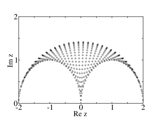
Figure 1: The partition function zeroes for free Wilson fermions on a $40\times 40$ lattice, where $z=1/2\kappa$ is the inverse hopping parameter.

We generated zeroes for a wide range of lattices, and their distributions, as given by (6), are plotted in Fig. 2. The data collapses onto a universal curve which goes through the origin, indicating that (6) is indeed a suitable form for the density of zeroes and indicating the occurence of a phase transition. Fits close to the origin yield an exponent compatible with the expected value, $\alpha=0$. The error estimates appropriate to such a fit are non-trivial and we leave their discussion to a separate publication [9].

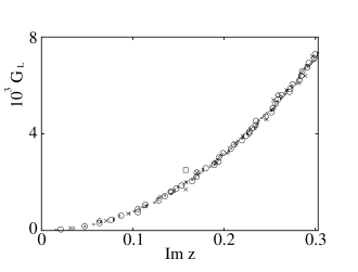
Figure 2: The distribution of zeroes for free Wilson fermions. The symbols   , $\diamond$, $\times$,    and    correspond to square lattices of length $L=20$, 50, 100, 150, and 200, respectively.

4 CONCLUSIONS

A new method to extract the (continuous) density of zeroes from (discrete) finite-size data has been extended to deal with the case of two-dimensional distributions of zeroes and systems in which the zeroes occur in degenerate sets. The method has been demonstrated in an application to the free Wilson fermion model and seen to be capable of direct determination of the strength of the phase transition as measured by the critical exponent $\alpha$.

References

- [1] W. Janke and R. Kenna, J. Stat. Phys. 102 (2001) 1211; in: Computer Simulation Studies in Condensed-Matter Physics XIV, eds. D.P. Landau, S.P. Lewis, and H.-B. Schüttler (Springer, Berlin, 2002), p. 97.
- [2] W. Janke and R. Kenna, Nucl. Phys. B (Proc. Suppl.) 106-107 (2002) 905; Comp. Phys. Comm. 147 (2002) 443.
- [3] N.A. Alves, J.P.N. Ferrite, and U.H.E. Hansmann, Phys. Rev. E 65 (2002) 036110; N.A. Alves, U.H.E. Hansmann, and Y. Peng, Int. J. Mol. Sci. 3 (2002) 17.
- [4] W. van Saarlos and D. Kurtze, J. Phys. A 17 (1984) 1301; J. Stephenson and R. Couzens, Physica 129A (1984) 201.
- [5] B. Derrida, Phys. Rev. B 24 (1981) 2613; V. Matveev and R. Shrock, J. Phys. A 28 (1995) 5235.
- [6] R. Abe, Prog. Theor. Phys. 38 (1967) 322; M. Suzuki, Prog. Theor. Phys. 38 (1967) 1243.
- [7] J. Stephenson, J. Phys. A 20 (1997) 4513.
- [8] R. Kenna, C. Pinto, and J.C. Sexton, Nucl. Phys. B (Proc. Suppl.) 83 (2000) 667; Phys. Lett. B 505 (2001) 125; R. Kenna and J.C. Sexton, Phys. Rev. D 65 (2002) 014507.
- [9] W. Janke, D. Johnston, and R. Kenna, in preparation.