One loop calculation of the renormalized anisotropy for improved anisotropic gluon actions on a lattice

Abstract

Using the infrared dispersion relation of the on shell gluon, we calculate the renormalisation of the anisotropy, $\chi$, to one loop in perturbation theory for lattice Yang–Mills theories, including the Wilson action and actions with Symanzik and/or tadpole improvement. Using twisted boundary conditions as a gauge invariant infrared regulator, we show for an SU(3) gauge group in $D=3+1$ dimensions that the one loop anisotropy is accurate to $O(3\%)$ for a range of $g^{2}$ and $\chi$ covering current simulations. In doing so we also present Feynman rules for SU(N) gauge groups with generic anisotropy structure (including ‘$3+1$’ and ‘$2+2$’ cases) for both twisted and untwisted boundary conditions.

I Introduction

Lattice Monte Carlo simulations operate by dividing a finite volume of space and time into a grid, such that in a given direction, $\mu$, we have $L_{\mu}$ points distance $a_{\mu}$ apart. The desire to obtain results free from uncontrolled finite volume contamination dictates that the product $a_{\mu}L_{\mu}$ be chosen to be suitably large in spatial directions (3 fm is often quoted for QCD). Controlling discretization effects similarly requires that $a_{\mu}$ be suitably small, but this must be balanced with the computational overhead that increases with $L_{\mu}$. Reducing the dependence of simulation results on the lattice spacing is clearly advantageous, and so–called (Symanzik) improved actions may achieve this, permitting the use of coarser lattices without increasing discretization effects lepage96 .

In many cases, lattice results (such as hadron masses or decay constants) are obtained from the decay of correlation functions, $C(\tau)$, over a range of temporal separations, $\tau$. It is a feature of such correlation functions that the signal to noise ratio decreases with increasing $\tau$, and beyond some $\tau_{c}$ measurements are dominated by statistical fluctuations. The precise value of $\tau_{c}$ depends upon many factors, including the operators correlated and the number of Monte Carlo measurements made, but appears to be relatively insensitive to the temporal lattice spacing, $a_{t}$. As measurements can only be made for $\tau$ an integer multiple of $a_{t}$, if the temporal lattice spacing is large compared to $\tau_{c}$ it will be hard to obtain an accurate picture of $C(\tau<\tau_{c})$. Improving the action does not help in this respect, and in addition, the inclusion of improvement in the temporal direction leads to the introduction of spurious (sometimes called ‘ghost’) poles in the gluonic propagator lepage96 . By not temporally improving the action we avoid this, but at the cost of increased discretization errors for given $a_{t}$. Controlling these, and the desire for increased temporal resolution of correlation functions, argues for the use of a small $a_{t}$.

We are thus motivated to choose a temporal lattice spacing that is smaller than the spatial, $a_{s}$, and such ‘anisotropic’ lattices can be created by tuning action couplings in the temporal direction differently to those in the spatial karsch82 . Anisotropic actions have already been successfully applied in many situations, including the glueball spectrum MP , the spectrum of excitations of the inter-quark potential JKM , heavy hybrids maea1 ; drea0 , and the fine structure of the quarkonium spectrum maea0 . More recently, anisotropic lattices have been shown to be very successful in nonrelativistic QCD (NRQCD) studies of two– and three–point correlators and finite momentum hadrons and semileptonic $B$ decays shigemitsu01 ; shigemitsu02 .

A more widespread use has been hampered by the fact that the bare anisotropy (or aspect ratio) in the simulated action, $\chi=a_{s}/a_{t}$, is not, due to quantum mechanical effects, the same as the measured value, $\chi_{R}$. Typically, we wish to estimate the continuum limit ratio of a mass, $M$, to a given scale, $K$, using the lattice measurements, $\hat{M}$ (in units of $a_{t}$) and $\hat{K}$ (often derived from the static quark potential, and in units of $a_{s}$) respectively. Up to finite lattice spacing corrections,

$$\frac{M}{K}=\frac{\hat{M}}{\chi_{R}\hat{K}}\;.$$ (1)

We thus require $\chi_{R}$, and with a sufficiently small error that this does not represent the dominant uncertainty in the final estimate. $\chi_{R}$ may be measured in Monte Carlo simulations, e.g. alea , but it is an expensive calculation which must be repeated for every choice of the bare couplings.

More generally, (lattice) perturbation theory may be used to calculate the renormalisation of quantities, and it is well known that with ‘tadpole improvement’ such calculations converge quickly to the measured data at simulated values of the gauge coupling, $g^{2}$, lepage96 . In this paper we obtain $Z(g^{2},\chi)\equiv\chi_{R}/\chi$ to one loop for a wide range of anisotropies for SU(3) gauge theories in four dimensions. We focus on the Wilson action and a commonly used Symanzik improved action. Our results apply both to actions with and without tadpole improvement; in the Wilson case we cover both plaquette and (Landau) mean link improvement, whilst in the Symanzik improved case we discuss here only the mean link improved case.

These is no reason, a priori, why the lattice spacing should be identical in all spatial directions, and indeed there are situations where we might choose this not to be the case. A typical example is where increased momentum resolution is desired for correlation functions of operators at finite momentum. Rather than increase the computational overhead by a global rescaling, $a$ can be made smaller in one spatial direction burgio02 . Whilst we do not consider calculations for this case explicitly in this paper, when we describe the Feynman rules in Section II, we allow for arbitrary anisotropic lattice structure as well as general actions. We use twisted boundary conditions as a gauge invariant infrared regulator. In Section III we describe our calculation of the anisotropy from the dispersion relation of the on shell gluon propagator. We compare these one loop results to measurements of $\chi_{R}$ from simulations, and show that the one loop result is accurate to within 3–4% over the range of couplings covered by Monte Carlo simulations. Finally, in Section IV we provide a summary of our findings and some conclusions.

II The Perturbation Theory

It is useful to consider the derivation of an anisotropic lattice action from the isotropic continuum theory in two stages. We first obtain an action for an anisotropic continuum, which is then discretized.

II.1 continuum anisotropy

The starting point, and the fixed point of the lattice action, is a $D$–dimensional continuum field theory in an Euclidean space-time that is invariant under Lorentz transformations and hence isotropic. We may choose to change our measurement units in the continuum theory, and by different factors in different directions, which leads to the introduction of an anisotropy factor (or factors), $\chi$, into the action, being the ratio of the length units in different directions. Nonetheless, Ward identities (derived by considering anisotropies differing infinitesimally from unity) can be enforced to ensure that the underlying theory maintains the correct Lorentz invariance under renormalisation.

We distinguish quantities in the isotropic theory from those in the anisotropic by the use of ‘hats’ in the former case. Although the original metric is

$$\hat{\mathfrak{g}}_{\alpha\beta}={\rm diag}(+1,+1,...,+1),$$ (2)

we find it convenient to introduce the notation of covariant and contravariant indices. The contraction of a momentum and position , $\hat{{\bf p}}\cdot\hat{{\bf x}}\equiv\hat{p}_{\alpha}\hat{x}^{\alpha}$, must be invariant under rescaling, i.e.

$$\hat{p}_{\alpha}\hat{x}^{\alpha}=p_{\mu}x^{\mu}.$$ (3)

We can relate the rescaled fields to the original by the use of a set of vierbeins

$$x^{\mu}={e^{\mu}}_{\alpha}\hat{x}^{\alpha}\;,~{}~{}~{}~{}p_{\mu}={e_{\mu}}^{\alpha}\hat{p}_{\alpha}\;.$$ (4)

The metric in these variables is

$$\mathfrak{g}_{\mu\nu}={e_{\mu}}^{\alpha}{e_{\nu}}_{\alpha}\;,~{}~{}~{}~{}\mathfrak{g}\equiv\det\mathfrak{g}_{\mu\nu}\;.$$ (5)

In the most general case there will be $D-1$ anisotropy factors, but for the rescaling in the temporal direction only, as we consider in this paper,

$${e^{\mu}}_{\alpha}=\left(\chi,1,...,1\right)\;,~{}~{}~{}~{}{e_{\mu}}^{\alpha}=\left(\frac{1}{\chi},1,...,1\right)\;,$$ (6)

and

$$\mathfrak{g}_{\mu\nu}={\rm diag}\left(\frac{1}{\chi^{2}},1,...,1\right)\;,~{}~{}~{}~{}\mathfrak{g}=\frac{1}{\chi^{2}}\;.$$ (7)

Using these conventions, the natural position vector is covariant under rescaling, $\hat{{\bf x}}=(\hat{x}^{\alpha})=(t,{\underline{x}})$, so the momentum must be contravariant $\hat{{\bf p}}=(\hat{p}_{\alpha})=(E,{\underline{p}})$ such that Eqn. (3) is satisfied. The volume element is given by

$$d\hat{{\bf x}}=d{\bf x}\prod_{\mu=1}^{D}{e_{\mu}}^{\alpha}=d{\bf x}\sqrt{\mathfrak{g}}=\frac{d{\bf x}}{\chi}.$$ (8)

The dimensionfull (colour) vector potential and derivatives behave as $\hat{{\bf p}}$, and so the Yang–Mills action becomes

$$S_{\rm YM}=\frac{1}{4}\int d\hat{{\bf x}}\hat{F}_{\alpha\beta}\hat{F}^{\alpha\beta}=\frac{1}{4}\int d{\bf x}\sqrt{\mathfrak{g}}\>F_{\alpha\beta}F^{\alpha\beta}=\frac{1}{4}\int d{\bf x}\sqrt{\mathfrak{g}}\>\mathfrak{g}^{\mu\sigma}\mathfrak{g}^{\nu\tau}F_{\mu\nu}F_{\sigma\tau}\;.$$ (9)

For the specific example above,

$$S_{\rm YM}=\frac{1}{4}\int\frac{d{\bf x}}{\chi}\left({\chi}^{2}F_{0i}F_{0i}+F_{ij}F_{ij}\right)\;.$$ (10)

II.2 the propagator

To construct the Feynman diagrams for any action the gluon propagator must be computed. This is done for a given momentum by inverting the two-point gluon vertex, which for the isotropic (continuum) case is given by $\hat{V}^{(2)\alpha\beta}(\hat{{\bf k}})=\hat{k}_{\epsilon}\hat{k}^{\epsilon}\delta^{\alpha\beta}-\hat{k}^{\alpha}\hat{k}^{\beta}$. Before this can be done the gauge must be fixed and we add to the action a gauge fixing term and source, which in momentum space appear as

$$S_{\rm g.f.}=\int\frac{d\hat{{\bf k}}}{(2\pi)^{4}}\>\frac{1}{2\alpha}\hat{A}_{\mu}(\hat{{\bf k}})\hat{k}^{\mu}\hat{k}^{\nu}\hat{A}_{\nu}(-\hat{{\bf k}})-\hat{J}^{\mu}(\hat{{\bf k}})\hat{A}_{\mu}(-\hat{{\bf k}})\,.$$ (11)

The parameter $\alpha$ is the usual gauge-fixing parameter and, for example, $\alpha=1$ corresponds to Feynman gauge. In moving to the anisotropic theory, $d\hat{{\bf k}}=d{\bf k}/\sqrt{\mathfrak{g}}$, which affects functional derivatives with respect to the anisotropic source, $J^{\mu}$. We can rescale $A_{\mu}$ to absorb this metric factor, which multiplies terms quadratic in $A_{\mu}$ by $\sqrt{\mathfrak{g}}$. The two point function, $V^{(2)\mu\nu}({\bf k})$, that we shall shortly derive from the action, will already contain this factor and the inverse propagator becomes

$$\Gamma^{(\alpha)\mu\nu}({\bf k})=V^{(2)\mu\nu}({\bf k})+\frac{k^{\mu}k^{\nu}}{\alpha}\sqrt{\mathfrak{g}}\;.$$ (12)

By illustration, the inverse propagator in the continuum for $\alpha=1$ has the form

$$\Gamma^{(\alpha=1)\mu\nu}({\bf k})=\delta^{\mu\nu}\sqrt{\mathfrak{g}}k_{\rho}k^{\rho}=\frac{\delta^{\mu\nu}}{\chi}\left(\chi^{2}{\hat{k}_{0}}^{2}+\sum_{i}{\hat{k}_{i}}^{2}\right)$$ (13)

where the latter expression uses the isotropic momenta, which for a lattice theory we shall equate to the ‘physical’ ones.

The propagator is

$$G^{(\alpha)}_{\mu\nu}=\left({\Gamma^{(\alpha)\mu\nu}}\right)^{-1}\;.$$ (14)

To fix to Landau gauge we must be more careful. Consider the case where we wish to change the gauge from $\alpha$ to $\gamma$ after inversion. Then

$$\Gamma^{(\gamma)\mu\nu}=\Gamma^{(\alpha)\mu\nu}+\left(\frac{1}{\gamma}-\frac{1}{\alpha}\right)k^{\mu}k^{\nu}\sqrt{\mathfrak{g}}\;.$$ (15)

We write

$$G^{(\gamma)}_{\mu\nu}=G^{(\alpha)}_{\mu\nu}+D_{\mu\nu}\;,$$ (16)

and then $D_{\mu\nu}$ satisfies

$$\left(\Gamma^{(\alpha)\mu\nu}+\left(\frac{1}{\gamma}-\frac{1}{\alpha}\right)k^{\mu}k^{\nu}\sqrt{\mathfrak{g}}\right)\left(G^{(\alpha)}_{\nu\rho}+D_{\nu\rho}\right)={\delta^{\mu}}_{\rho}\;.$$ (17)

The solution for $D_{\mu\nu}$ is

$$D_{\mu\nu}=-\frac{(\alpha-\gamma)}{\sqrt{\mathfrak{g}}}{k_{\mu}k_{\nu}\over(k_{\alpha}k^{\alpha})^{2}}\;.$$ (18)

II.3 discretization

The anisotropically formulated theory may be discretized in the normal way, and in these anisotropic units we set the lattice spacing, $a$, to be the same in each direction.

On a cubical lattice $\Lambda_{D}$ in dimension $D$ (with ${\bf x}\in\Lambda_{D}$, $\mu=1,\ldots,D$) the gauge field is denoted $U$,

$$U=\left\{U_{\mu}({\bf x}):~{}U_{\mu}({\bf x})\in SU(N)\right\}\;,$$ (19)

where $U_{\mu}({\bf x})$ is associated with the link $({\bf x},\mu)$.

We define the perturbative gauge field $A$ by

$$A=\left\{A_{\mu}({\bf x}+{\textstyle{1\over 2}}{\bf e}_{\mu}):~{}A_{\mu}({\bf x}+{\textstyle{1\over 2}}{\bf e}_{\mu})\in alg(SU(N))\right\}\;,$$ (20)

with ${\bf e}_{\mu}$ the lattice basis vectors, all of unit length and changing covariantly with rescaling. Expanding in the colour index, $a$,

$$A_{\mu}=A_{\mu}^{a}\,T_{a}\;,~{}~{}~{}[T_{a},T_{b}]=-f_{abc}T_{c}\;,~{}~{}~{}\mbox{Tr}(T_{a}T_{b})=-{\textstyle{1\over 2}}\,\delta_{ab}\;,$$ (21)

where $T_{a}$ are the (anti-hermitian) generators of $SU(N)$ with structure constants $f_{abc}$. It is expedient to associate the gauge potential with the centre of the link, and then

$$U_{\mu}({\bf x})=\exp(gA_{\mu}({\bf x}+{\textstyle{1\over 2}}{\bf e}_{\mu}))\;,$$ (22)

where $g$ is the bare coupling constant, and we have absorbed a factor of $a$ into each component of $A_{\mu}$.

For a lattice with $L_{\mu}$ sites in the $\mu$ direction the momentum vector ${\bf k}$ is

$${\bf k}=\frac{2\pi}{a}\,({\bar{k}_{1}\over L_{1}},\ldots,{\bar{k}_{D}\over L_{D}})\;,~{}~{}0\leq\bar{k}_{\mu}<L_{\mu}\;,~{}~{}\bar{k}_{\mu}\in\mathbb{Z}\;,$$ (23)

and the sum over ${\bf k}$ stands for the sum over the components $\bar{k}_{\mu}$. In the limit that $L_{\mu}\rightarrow\infty$ we have

$$\frac{1}{aL_{\mu}}\sum_{\bar{k}_{\mu}}~{}\rightarrow~{}\int\frac{dk_{\mu}}{2\pi}\;.$$ (24)

The Fourier transform to momentum space is

$$\tilde{A}_{\mu}({\bf k}) = \sum_{\bf x}\,e^{-i{\bf k}\cdot({\bf x}+{1\over 2}{\bf e}_{\mu})}A_{\mu}({\bf x}+{\textstyle{1\over 2}}{\bf e}_{\mu}),$$

$$A_{\mu}({\bf x}+{\textstyle{1\over 2}}{\bf e}_{\mu}) = {1\over V}\sum_{\bf k}\,e^{i{\bf k}\cdot({\bf x}+{1\over 2}{\bf e}_{\mu})}\tilde{A}_{\mu}({\bf k})\;,$$ (25)

where $V=\prod_{\mu}L_{\mu}$ is the number of lattice points. It is useful to re-express the position of a gauge potential as $\mbox{\boldmath$v$}_{\mu}=2({\bf x}+{\textstyle{1\over 2}}{\bf e}_{\mu})$, which is a $D$–dimensional vector with integer (covariant) components.

II.4 vertex functions

To permit us to compute perturbation theory for a range of actions, we have developed an algorithmic method for expanding a general gauge theory action on a lattice in an appropriate form for perturbative calculations to be carried out. The approach follows closely the method and notation of Lüscher and Weisz luwe but is extended to accommodate, inter alia, anisotropy, fermionic actions, actions for non-relativistic heavy quarks (NRQCD) and more complicated definitions of the action in the purely gluonic sector. The algorithm is implemented in the Python programming language. For the work presented in this paper we briefly review the notation relevant to the present calculation and refer to luwe for further information.

The lattice action for the pure glue sector can be written as a sum over contours

$$S[U]=\sum_{{\bf x},\alpha}~{}c_{\alpha}\>\mathrm{Re}\>\mbox{Tr}\;(P_{\alpha}(U;{\bf x}))\;,$$ (26)

which is defined in terms of the coupling constants, $c_{\alpha}$, and the $P_{\alpha}$, which are closed Wilson loops.

The perturbative action is the expansion of $S[U]$ as a polynomial in $A$ and the coefficients of the monomials will determine the vertices of the theory. We denote this action as $S[A]$ and following luwe we write

$$S[A]=\sum_{r}{g^{r}\over r!}\;\sum_{{\bf k}_{1},\mu_{1},a_{1}}\ldots\sum_{{\bf k}_{r},\mu_{r},a_{r}}\tilde{A}^{a_{1}}_{\mu_{1}}({\bf k}_{1})\ldots\tilde{A}^{a_{r}}_{\mu_{r}}({\bf k}_{r})\;V_{r}({\bf k}_{1},\mu_{1},a_{1};\,\ldots;\,{\bf k}_{r},\mu_{r},a_{r})\;.$$ (27)

By a choice of units we set the lattice spacing to $a=1$. The value of the lattice spacing in physical units is determined by a calculation of a physical dimensionfull quality and depends on $g$ and hence on the renormalized coupling constant through the standard $\beta$ function. Other quantities, such as the bare anisotropy, are determined by the coupling coefficients $c_{\alpha}$.

The Euclidean Feynman rule for the $r$-point gluon vertex function is $(-g^{r}V_{r})$, where the vertex $V_{r}$ can be expressed as luwe

$$V_{r}({\bf k}_{1},\mu_{1},a_{1};\,\ldots;{\bf k}_{r},\mu_{r},a_{r})=\sum_{\sigma\in{\cal S}_{r}}\sigma\cdot C_{r}(a_{1},\ldots,a_{r})~{}\sigma\cdot Y_{r}({\bf k}_{1},\mu_{1};\,\ldots;{\bf k}_{r},\mu_{r})\;,$$ (28)

where we symmetrize over ${\cal S}_{r}$, the permutation group of $r$ objects.

The $C_{r}$ are the Clebsch-Gordan coefficients which, owing to the reality of the action, are defined by

$$C_{r}(a_{1},\ldots,a_{r})=\mbox{Tr}\;(T_{a_{1}}\ldots T_{a_{r}})+(-1)^{r}\mbox{Tr}\;(T_{a_{r}}\ldots T_{a_{1}})\;.$$ (29)

Under ${\cal Z}_{r}$, the subgroup of cyclic permutations and inversion, the $C_{r}$ have simple properties,

$$\sigma\cdot C_{r} = \chi_{r}(\sigma)\;C_{r}~{}~{}~{}~{}\sigma\in{\cal Z}_{r},$$

$$\chi_{r}(\sigma) = \left\{\begin{array}[]{l}1~{}~{}~{}\mbox{for~{}~{}}\sigma\mbox{~{}~{}a cyclic permutation},\\ (-1)^{r}~{}~{}~{}\mbox{for~{}~{}}\sigma\mbox{~{}~{}the inversion,}\end{array}\right.$$ (32)

so it is useful to split the symmetrization operation into two steps

$$V_{r}({\bf k}_{1},\mu_{1},a_{1};\,...;\,{\bf k}_{r},\mu_{r},a_{r}) = \sum_{\sigma\in{\cal S}_{r}/{\cal Z}_{r}}\sigma\cdot C_{r}(a_{1},...,\alpha_{r})~{}\sigma\cdot Y_{r}({\bf k}_{1},\mu_{1};\,...;\,{\bf k}_{r},\mu_{r})\;,$$

$$Y_{r} = \sum_{\alpha}Y^{\alpha}_{r}\;,~{}~{}~{}~{}Y^{\alpha}_{r}=\sum_{\sigma\in{\cal Z}_{r}}\;\chi_{r}(\sigma)\>\sigma\cdot\bar{Y}^{\alpha}_{r}\;.$$ (33)

The symmetrization over ${\cal Z}_{r}$ is carried out within the Python vertex generation code, whereas any remaining permutations (for $r\geq 4$) must be carried out during the loop integration. $\bar{Y}^{\alpha}_{r}$ is the contribution from the Wilson loop $P_{\alpha}$ given by a sum of $n_{r}$ terms with the same momentum and Lorentz structure

$$\bar{Y}^{\alpha}_{r}({\bf k}_{1},\mu_{1};\ldots;{\bf k}_{r},\mu_{r})=c_{\alpha}\sum_{n=1}^{n_{r}}\frac{f^{\alpha}_{n}}{2r!}\;\exp\left(\>\frac{i}{2}\left({\bf k}_{1}\cdot\mbox{\boldmath$v$}^{n}_{1}+\ldots+{\bf k}_{r}\cdot\mbox{\boldmath$v$}^{n}_{r}\right)\right)\;.$$ (34)

The factor of $(r!)$ normalises the symmetrization, and the dependence on the Lorentz indices $\mu_{1},\ldots,\mu_{r}$ has been suppressed. The prefactor of $\frac{1}{2}$ normalises Eqn. (29). The expansion of $S[U]$ can thus be represented as a set of ‘entities’ $[f_{n};\mbox{\boldmath$v$}^{n}_{1},\ldots,\mbox{\boldmath$v$}^{n}_{r}]$, $n=1,\ldots,n_{r}$, where $f_{n}$ is an amplitude which is an integer for simple actions. The Python code produces data files where these are appropriately labelled so that, given the Lorentz indices $(\mu_{1},\ldots,\mu_{r})$ and the incoming momenta ${\bf k}_{1},\ldots,{\bf k}_{r}$, the corresponding value of the $r$-point vertex function $V_{r}$ can be computed. The relevant Feynman diagrams can be constructed and the integrals over loop momenta performed either by direct summation over modes or using numerical integration routines. The gluon $r$-point functions are generated with the anisotropy fixed at the chosen (bare) value, and thus encoded in the amplitudes, $f$. We find this allows greater simplification of the data files produced by the Python and more efficient loop integral evaluation code. The time taken to rerun the vertex generation code for different $\chi$ is negligible, especially when offset against this. A more complete description of the implementation may be found in lat02 ; meanlink02 .

The gluonic propagator is derived as per the continuum theory, using the two point vertex for the particular action, $V_{2}({\bf k},\mu;-{\bf k},\nu)$, and pairs of forward and backward nearest neighbour difference operators,

$$\hat{\Delta}_{\alpha} = (\Delta_{0},\Delta_{i})~{}~{}~{}\Rightarrow~{}~{}~{}\Delta_{\mu}=(\frac{\Delta_{0}}{\chi},\Delta_{i})\;,~{}~{}~{}\Delta^{\mu}=(\chi\Delta_{0},\Delta_{i})\;,$$

$$\hat{\Delta}^{2} = \hat{\Delta}^{\pm}_{\alpha}\hat{\Delta}^{\mp\alpha}=\hat{\Delta}^{\pm}_{0}\hat{\Delta}^{\mp}_{0}+\sum_{i}\hat{\Delta}^{\pm}_{i}\hat{\Delta}^{\mp}_{i}\;.$$ (35)

to replace the position space derivatives in the gauge fixing term. The difference operators are

$$\hat{\Delta}^{+} = f({\bf x}+\hat{\mbox{\boldmath$\mu$}})-f({\bf x})$$

$$\hat{\Delta}^{-} = f({\bf x})-f({\bf x}-\hat{\mbox{\boldmath$\mu$}})$$ (36)

for some $f({\bf x})$. The net effect is merely to replace momentum components, $p_{\mu}$, prior to any raising of the index, by $\tilde{p}_{\mu}\equiv 2\;\hbox{sin}(p_{\mu}/2)$ in Eqns. (12–18).

II.5 Faddeev–Popov ghosts

The Faddeev–Popov ghost term is of the form $S_{\rm ghost}=\int d{\bf x}\>{\bar{\eta}}^{a}M^{ab}\eta^{b}\;$, where ${\bar{\eta}}$ and $\eta$ are the usual adjoint anti-commuting ghost fields. The ghost fields are not observable, and form only internal lines in Feynman diagrams. We are thus free to choose the normalisation of the fields such that explicit factors of $\sqrt{\mathfrak{g}}$ do not appear in the momentum space Feynman rules for the ghosts. The anisotropy then only appears implicitly in the raising of indices.

The Faddeev–Popov matrix $\Delta^{ab}$ is determined by the gauge fixing condition corresponding to the choice of gauge in the propagator. The gauge-fixing is done by introducing the identity in the form

$$1=\int d\alpha\;\int\prod dA_{\mu}\;\delta(F[A_{\mu}]-\lambda)\exp(-\lambda^{2}/2\alpha)\;.$$ (37)

We use the linear gauge function $(F[A_{\mu}]={(\Delta^{-})}^{\mu}A_{\mu}$ and, as is well known, the matrix $\Delta^{ab}$ is independent of $\alpha$ in this case. We denote the gauge transformation field by

$$g({\bf x})=\exp(\omega({\bf x}))\;,$$ (38)

where $\omega({\bf x})=\omega_{a}({\bf x})T^{a}$. For infinitesimal $\omega$ the gauge field transforms as

$$A^{\omega\;a}_{\mu} = A^{a}_{\mu}+\Omega^{a}_{\mu}-{g\over 2}{\bar{A}}^{ab}_{\mu}\Omega^{+\;b}_{\mu}~{}+~{}\sum_{n=2}^{\infty}\;g^{n}\alpha_{n}({\bar{A}}^{n}_{\mu})^{ab}\cdot\Omega^{b}_{\mu}\;.$$

$$\Omega_{\mu} = -\Delta^{+}_{\mu}\omega\;,~{}~{}~{}\Omega^{+}_{\mu}=(2+\Delta^{+}_{\mu})\omega\;,$$ (39)

where ${\bar{A}}_{\mu}$ is the adjoint representation for the gauge field and $\alpha_{n}$ is the coefficient of $x^{n}$ in the expansion of

$$b(x)={x\over e^{x}-1}=\sum_{n=0}^{\infty}\alpha_{n}x^{n}\;.$$ (40)

The Faddeev–Popov matrix is then

$$M^{ab}[A_{\mu}] = \left.{\delta F[A^{\omega\;a}_{\mu}]\over\delta\omega^{b}}\right|_{\omega=0}$$ (41)

$$= {(\Delta^{-})}^{\mu}\left[-\Delta^{+}_{\mu}\delta^{ab}-{g\over 2}{\bar{A}}^{ab}_{\mu}(2+\Delta^{+}_{\mu})-\sum_{n=2}^{\infty}\;g^{n}\alpha_{n}({\bar{A}}^{n}_{\mu})^{ab}\Delta^{+}_{\mu}\right]\;.$$

The inverse ghost propagator is given by the $O(g^{0})$ term and is

$$\Delta^{ab}({\bf x},{\bf y})=-\delta^{ab}\Delta^{2}({\bf x},{\bf y})\;,$$ (42)

giving rise to the standard $1/p^{2}$ ghost propagator.

The one-gluon vertex is given by the $O(g)$ term which gives the contribution to the action

$$g{\bar{\eta}}^{a}f^{abc}{(\Delta^{-})}^{\mu}\left(A^{b}_{\mu}(1+\Delta^{+}_{\mu}/2)\eta^{c}\right)\;,$$ (43)

and, integrating by parts, we get

$$-g({(\Delta^{+})}^{\mu}{\bar{\eta}}^{a})f^{abc}A^{b}_{\mu}\eta^{c}-{\textstyle{1\over 2}}g({(\Delta^{+})}^{\mu}{\bar{\eta}}^{a})f^{abc}(\Delta^{+}_{\mu}\eta^{c})\;.$$ (44)

The first term generates the standard three-point vertex that one expects from the continuum but the second term is a lattice artifact which is suppressed by a power of the lattice spacing $a$ as we should expect.

At order $g^{2}$ there is a two-gluon vertex which, using $\alpha_{2}=1/12$, can be read from Eqn. (41) to be

$${g^{2}\over 12}({(\Delta^{+})}^{\mu}{\bar{\eta}}^{a})\>A^{d}_{\mu}A^{e}_{\mu}\>f^{dac}f^{ecb}\>(\Delta^{+}_{\mu}\eta^{b})\;.$$ (45)

Higher order vertices follow a similar pattern but do not contribute to the one loop calculation we are considering.

II.6 the Haar measure

The field measure in the function integral is the Haar measure for integration over the lattice fields $U_{\mu}({\bf x})$ which take values in the Lie group. For the perturbative calculation this measure is re-expressed as the measure for the fields $A_{\mu}({\bf x})$, which take values in the Lie algebra, times a Jacobian which can be expanded perturbatively and included as counter terms in the perturbative action. We relate the infinitesimal vectors $d\xi=d\xi_{a}T^{a}$ and $dA=dA_{a}T^{a}$ in the fundamental representation of the Lie algebra by

$$e^{g\,d\xi}=e^{-gA}\;e^{g\,(A+dA)}$$ (46)

from which we derive the relation

$$dA^{a}=b(g{\bar{A}})^{ab}d\xi^{b}$$ (47)

where again ${\bar{A}}$ is in the adjoint representation and the function $b(x)$ is defined in Eqn. (40) above. The Haar measure is

$$\prod_{\mu,{\bf x}}d\xi_{\mu}({\bf x})=\prod_{\mu,{\bf x}}{\partial\xi_{\mu}({\bf x})\over\partial A_{\mu}({\bf x})}\;\prod_{\mu,{\bf x}}dA_{\mu}({\bf x})\;.$$ (48)

The Jacobian then leads to the term in the action

$$S_{\rm meas}=-\int\>d{\bf x}\>\sum_{\mu}\>\mbox{Tr}\left[\log b(g{\bar{A}}_{\mu}({\bf x}))\right]=\sum_{n=0}^{\infty}\;g^{n}\>\beta_{n}\int\>d{\bf x}\sum_{\mu}\>\mbox{Tr}\left({\bar{A}}_{\mu}^{n}({\bf x})\right)\;.$$ (49)

Noting that

$$-x{d\over dx}\log b(x)=b(x)\;,$$ (50)

we find that $\beta_{n}=\alpha_{n}/n$ with $\alpha_{n}$ the coefficients in the expansion of $b(x)$ defined in Eqn. (40).

The $O(g^{2})$ vertex from the measure relevant to the one loop calculation is then

$${1\over 8}\int\>d{\bf x}\>\sum_{a,\mu}\>[A^{a}_{\mu}({\bf x})]^{2}\;.$$ (51)

II.7 twisted boundary conditions

We follow Lüscher and Weisz and use twisted periodic boundary conditions for the gauge field. There is then no zero mode and hence no concomitant infrared divergences in the gluon self energy whilst gauge invariance is maintained. We briefly review these boundary conditions and refer to luwe for further details.

For an orthogonal twist the twisted boundary condition for gauge fields is

$$U_{\mu}({\bf x}+L_{\nu}{\bf e}_{\nu})=\Omega_{\nu}U_{\mu}({\bf x})\Omega^{-1}_{\nu}\;,$$ (52)

where the twist matrices $\Omega_{\nu}$ are constant $SU(N)$ matrices which satisfy

$$\Omega_{\mu}\Omega_{\nu}=z_{\mu\nu}\Omega_{\nu}\Omega_{\mu}$$ (53)

and $z_{\mu\nu}=\exp(2\pi in_{\mu\nu}/N)$ is an element of the centre of SU(N) with $n_{\mu\nu}=0,1,\ldots,N-1$. The particular boundary conditions imposed are uniquely specified by the antisymmetric integer tensor $n_{\mu\nu}$ and a complete discussion may be found in gonzalez97 . The condition that the twist be orthogonal is that $n_{\mu\nu}\tilde{n}_{\mu\nu}=0~{}\mbox{mod}N$, where $\tilde{n}_{\mu\nu}=\epsilon_{\mu\nu\sigma\rho}n_{\sigma\rho}$. The gauge potential $A_{\mu}({\bf x})$ also satisfies the periodicity condition in Eqn. (52).

Following luwe we choose $n_{\mu\nu}=0$ everywhere, save $n_{12}=-n_{21}=1$. $\Omega_{1}$ and $\Omega_{2}$ are then determined up to a unitary $SU(N)$ transformation and $\Omega_{3}=\Omega_{4}={1}$. In the case of orthogonal twist $\Omega_{3}$, $\Omega_{4}$ can be expressed in terms of $\Omega_{1}$ and $\Omega_{2}$ once the values of $n_{\mu\nu}$ are given. This will affect the momentum spectrum in the $3,4$-directions, but the Feynman rules given below are unchanged.

The lattice is here taken to be continuous in the $3,4$-directions and of extent $L$ sites in the $1,2$-directions. The momentum spectrum, ${\bf k}$, is then continuous in $k_{3},k_{4}$ and discrete in $k_{1},k_{2}$ with

$$k_{i}={2\pi\bar{k}_{i}\over L_{i}}+{2\pi n_{i}\over NL_{i}},~{}~{}~{}~{}~{}i=1,2\;,~{}~{}~{}~{}~{}0\leq\bar{k}_{i}<L_{i},~{}~{}~{}~{}~{}0\leq n_{i}<N\;,~{}~{}~{}~{}~{}\bar{k}_{i},n_{i}\in\mathbb{Z}\;,$$ (54)

with $n_{1}=n_{2}=0$ excluded to eliminate the zero mode and impose a gauge-invariant infrared cutoff momentum of $2\pi/NL$. Negative momentum in these directions is $-k_{i}=(-\bar{k}_{i},-n_{i})$, adding appropriate multiples of $L$ and $N$ to remain in the ranges defined above.

The Fourier expansion of a colour field $\phi({\bf x})$ is

$$\phi({\bf x})={1\over NL_{1}L_{2}}\sum_{k_{1},k_{2}}\int\;{dk_{3}\over 2\pi}{dk_{4}\over 2\pi}\;e^{ik(x+{\scriptstyle{1\over 2}}{\bf e}_{\mu})}\Gamma({\mbox{\boldmath$n$}}){\tilde{\phi}}_{\mbox{\boldmath$\scriptstyle n$}}({\bf k})\;,$$ (55)

where ${\tilde{\phi}}_{\mbox{\boldmath$\scriptstyle n$}}({\bf k})$ is a scalar field and the sum over $k_{1},k_{2}$ signifies the sum is over $\bar{k}_{1},\bar{k}_{2}$ and the twist vector ${\mbox{\boldmath$n$}}\equiv(n_{1},n_{2})$. The $N^{2}-1$ $SU(N)$ matrices, $\Gamma({\mbox{\boldmath$n$}})$, are given in terms of $\Omega_{1},\Omega_{2}$ by

$$\Gamma({\mbox{\boldmath$n$}})=z^{(n_{1}+n_{2})(n_{1}+n_{2}-1)/2}\Omega_{1}^{-n_{2}}\Omega_{2}^{n_{1}}\;,$$ (56)

where $z=\exp(2i\pi/N)$ is an element of the centre of $SU(N)$. We do not need to construct the $\Gamma({\mbox{\boldmath$n$}})$ explicitly but only evaluate the trace algebra associated with the perturbative vertices. We introduce the coefficients

$$\gamma_{{\mbox{\boldmath$\scriptstyle n$}}a}=\mbox{Tr}(\Gamma^{\dagger}({\mbox{\boldmath$n$}})T_{a})\;,$$ (57)

for which we have the relations

$$\begin{array}[]{rcl}{2\over N}\gamma^{\dagger}_{a{\mbox{\boldmath$\scriptstyle n$}}}\gamma_{{\mbox{\boldmath$\scriptstyle n$}}b}&=&\delta_{ab}\;,\\ {2\over N}\gamma_{{\mbox{\boldmath$\scriptstyle n$}}a}\gamma^{\dagger}_{a{\mbox{\boldmath$\scriptstyle m$}}}&=&\delta_{{\mbox{\boldmath$\scriptstyle n$}}{\mbox{\boldmath$\scriptstyle m$}}}\;,\\ T_{a}&=&{1\over N}\Gamma({\mbox{\boldmath$n$}})\gamma_{{\mbox{\boldmath$\scriptstyle n$}}a}\;,\\ \Gamma({\mbox{\boldmath$n$}})&=&2T_{a}\gamma^{\dagger}_{a{\mbox{\boldmath$\scriptstyle n$}}}\;.\end{array}$$ (58)

In addition, for an adjoint field we can define the set of scalar fields labelled by $n$

$$\phi_{\mbox{\boldmath$\scriptstyle n$}}({\bf x})=\gamma_{{\mbox{\boldmath$\scriptstyle n$}}a}\phi_{a}~{}~{}\Rightarrow~{}~{}\phi({\bf x})={1\over N}\Gamma({\mbox{\boldmath$n$}})\phi_{\mbox{\boldmath$\scriptstyle n$}}({\bf x})\;.$$ (59)

Using Eqn. (55) $\phi_{\mbox{\boldmath$\scriptstyle n$}}({\bf x})$ has Fourier transform ${\tilde{\phi}}_{\mbox{\boldmath$\scriptstyle n$}}({\bf k})$. Note that the related scalar field

$$\bar{\phi}_{\mbox{\boldmath$\scriptstyle n$}}({\bf x})=e^{-2\pi i(n_{1}x_{1}+n_{2}x_{2})/NL}\phi_{\mbox{\boldmath$\scriptstyle n$}}({\bf x})\;,$$ (60)

is periodic on the lattice and has a momentum spectrum defined by the $\bar{k}_{i}$ in Eqn. (54) which allows the numerical Fourier transform to be easily computed.

Defining the symmetric and antisymmetric products of twist vectors

$$({\mbox{\boldmath$n$}},{\mbox{\boldmath$m$}}) = n_{1}m_{1}+n_{2}m_{2}+(n_{1}+m_{1})(n_{2}+m_{2})\;,$$

$$\langle{\mbox{\boldmath$n$}},{\mbox{\boldmath$m$}}\rangle = n_{1}m_{2}-n_{2}m_{1}\;,$$ (61)

the Clebsch-Gordan coefficients given in Eqn. (29) are modified to become

$$C^{TW}_{r}({\mbox{\boldmath$n$}}_{1},\ldots,{\mbox{\boldmath$n$}}_{r})=\frac{1}{N}\left(\mbox{Tr}(\Gamma({\mbox{\boldmath$n$}}_{1})\ldots\Gamma({\mbox{\boldmath$n$}}_{r}))~{}+~{}(-1)^{r}\mbox{Tr}(\Gamma({\mbox{\boldmath$n$}}_{r})\ldots\Gamma({\mbox{\boldmath$n$}}_{1}))\right)\;.$$ (62)

The $C^{TW}_{r}$ can be evaluated using the relations

$$\begin{array}[]{rcl}\Gamma({\mbox{\boldmath$n$}})&=&{1}~{}~{}~{}{\mbox{\boldmath$n$}}={\bf 0}~{}\mbox{mod}~{}N\;,\\ \mbox{Tr}(\Gamma({\mbox{\boldmath$n$}}))&=&0~{}~{}~{}{\mbox{\boldmath$n$}}\neq{\bf 0}~{}\mbox{mod}~{}N\;,\\ \Gamma({\mbox{\boldmath$n$}})^{\dagger}&=&z^{-{\scriptstyle{1\over 2}}({\mbox{\boldmath$\scriptstyle n$}},{\mbox{\boldmath$\scriptstyle n$}})}\Gamma(-{\mbox{\boldmath$n$}})\;,\\ \Gamma({\mbox{\boldmath$n$}}^{\prime})\Gamma({\mbox{\boldmath$n$}})&=&z^{{\scriptstyle{1\over 2}}(\langle{\mbox{\boldmath$\scriptstyle n$}}^{\prime},{\mbox{\boldmath$\scriptstyle n$}}\rangle-({\mbox{\boldmath$\scriptstyle n$}}^{\prime},{\mbox{\boldmath$\scriptstyle n$}}))}\Gamma({\mbox{\boldmath$n$}}^{\prime}+{\mbox{\boldmath$n$}})\;,\end{array}$$ (63)

where $({\mbox{\boldmath$n$}}~{}\mbox{mod}~{}N)$ is understood to apply to each component, $n_{1,2}$, and the argument of $\Gamma$ is evaluated $\mbox{mod}~{}N$. We then derive the useful result

$$C^{TW}_{r}(-{\mbox{\boldmath$n$}}_{1},\ldots,-{\mbox{\boldmath$n$}}_{r})=(-1)^{r}z^{-{\scriptstyle{1\over 2}}\sum_{i=1}^{r}({\mbox{\boldmath$\scriptstyle n$}}_{i},{\mbox{\boldmath$\scriptstyle n$}}_{i})}{C^{TW}_{r}}^{*}({\mbox{\boldmath$n$}}_{1},\ldots,{\mbox{\boldmath$n$}}_{r})\;.$$ (64)

For the inverse propagator we have

$$C_{2}^{TW}({\mbox{\boldmath$n$}},-{\mbox{\boldmath$n$}})=2z^{({\mbox{\boldmath$\scriptstyle n$}},{\mbox{\boldmath$\scriptstyle n$}})/2}\;.$$ (65)

The $r$-point vertex function is then given in a similar form to that in Eqn. (33) by

$$V_{r}({\bf k}_{1},\mu_{1};\,\ldots;\,{\bf k}_{r},\mu_{r})=\sum_{\sigma\in{\cal S}_{r}/{\cal Z}_{r}}\;\sigma\cdot C^{TW}_{r}({\mbox{\boldmath$n$}}_{1},\ldots,{\mbox{\boldmath$n$}}_{r})\;\sigma\cdot Y_{r}({\bf k}_{1},\mu_{1};\,\ldots;\,{\bf k}_{r},\mu_{r})\;.$$ (66)

Note that the momentum arguments ${\bf k}$ implicitly define the associated twist integers $n$. To simplify the notation, we replace in most subsequent expressions the twist vector with its ‘parent’ momentum, understanding that only the twist vector will contribute in functions such as $\Gamma({\bf k})$.

The structure of the vertex functions $Y_{r}$ is unaffected by the choice of boundary condition which is manifested only in the momentum spectrum used.

A simplifying feature is to note that all diagrams contributing to an $r$-point function carry the same overall phase factor from the centre of the gauge group. These phases can be taken out as overall factors and the remaining parts of the Clebsch-Gordan coefficients and propagator are real. The overall phase can be restored at the end of the calculation.

For the 3-point vertex on the left hand side of Fig. 1(a) we have (using momentum conservation ${\bf p}+{\bf k}+{\bf q}=0$)

$$C^{TW}_{3}(123) = {1\over N}\mbox{Tr}(\Gamma(-{\bf q}-{\bf p})[\Gamma({\bf q}),\Gamma({\bf p})]$$ (67)

$$= {1\over N}\mbox{Tr}(\Gamma({\bf q}+{\bf p})\Gamma(-{\bf q}-{\bf p}))\left(z^{{\scriptstyle{1\over 2}}(\langle{\bf q},{\bf p}\rangle-({\bf q},{\bf p}))}-z^{{\scriptstyle{1\over 2}}(\langle{\bf p},{\bf q}\rangle-({\bf p},{\bf q}))}\right)$$

$$= 2i\,\hbox{sin}\left({2\pi\over 3}\langle{\bf q},{\bf p}\rangle\right)z^{{\scriptstyle{1\over 4}}(({\bf q},{\bf q})+({\bf p},{\bf p})+({\bf q}+{\bf p},{\bf q}+{\bf p}))}.$$

In the diagram contributing to the gluon self energy of Fig. 1(a) the phase factors for both vertices are identical and, with the phases of internal lines, yields an overall phase of $z^{{\scriptstyle{1\over 2}}({\bf p},{\bf p})}$ as expected for a term in the self energy.

For the 4-point vertex loop of Fig. 1(b) there are three contributions from the permutations $S_{4}/{\cal Z}_{4}$ corresponding to $(1234)$, $(1243)$, $(1324)$ and in each case the $Y_{4}$ are real. We then find the Clebsch-Gordan factors to be

$$\begin{array}[]{rcl}C_{4}^{TW}(1234)&=&\begin{array}[]{rcl}C_{4}^{TW}(1243)&=&2z^{({\bf k},{\bf k})/2}z^{({\bf p},{\bf p})/2}\end{array}\\ \\ C_{4}^{TW}(1324)&=&2\hbox{cos}\>\left({2\pi\over 3}\langle{\bf k},{\bf p}\rangle\right)z^{({\bf k},{\bf k})/2}z^{({\bf p},{\bf p})/2},\end{array}$$ (68)

The $z^{({\bf k},{\bf k})/2}$ cancels the $z^{-({\bf k},{\bf k})/2}$ from the internal propagator giving an overall factor of $z^{({\bf p},{\bf p})/2}$ which is the expected phase.

II.8 ghost and measure Feynman rules

We choose the Fourier representation for the anti-ghost field ${\bar{\eta}}$ given in Eqn. (55) but use the conjugate twist matrices $\Gamma^{\dagger}(-{\mbox{\boldmath$n$}})$. In this case the ghost propagator is real and given by

$$\Delta({\bf p},-{\bf p})=\frac{1}{{\tilde{p}}_{\alpha}{\tilde{p}}^{\alpha}}\;.$$ (69)

Now consider the relevant part of the ${\bar{\eta}}A\eta$ vertex,

$$\int d{\bf x}\>f^{abc}{\bar{\eta}}^{a}A^{b}\eta^{c} = \int d{\bf x}\>2\mbox{Tr}({\bar{\eta}}[A,\eta])$$ (70)

$$= {2\over N^{3}}\mbox{Tr}(\Gamma^{\dagger}(-{\bf k})[\Gamma({\bf p}),\Gamma({\bf q})])\int d{\bf x}\>{\bar{\eta}}_{\bf k}A_{\bf p}\eta_{\bf q}\;.$$

where terms such as ${\bar{\eta}}_{\bf k}$ refer to the decomposition in Eqn. (59), with the momentum subscript restricted to the twist vector. The Clebsch-Gordan structure is

$$F_{3}({\bf k},{\bf p},{\bf q})=\mbox{Tr}(\Gamma^{\dagger}(-{\bf k})[\Gamma({\bf p}),\Gamma({\bf q})])=z^{-{\scriptstyle{1\over 2}}({\bf k},{\bf k})}C_{3}^{TW}({\bf k},{\bf p},{\bf q})$$ (71)

From the full structure of the ${\bar{\eta}}A\eta$ vertex in Eqn. (44) the momentum space Feynman vertex with momentum assignment shown in Fig. 1(c) is

$$-ig{\tilde{k}}^{\mu}\hbox{cos}\>(\frac{q_{\mu}}{2})F_{3}({\bf k},{\bf p},{\bf q})\;,$$ (72)

where there is no implied sum over $\mu$. Note that $C_{3}^{TW}({\bf k},{\bf p},{\bf q})$ plays the rôle of a structure constant. With a real ghost propagator this vertex contributes the same phase factor as does the 3-point gluon vertex and so it can be absorbed into the overall phase factor of the diagram.

The two-gluon vertex, Eqn. (45), can similarly be analysed. Assigning the ghost momentum ($-{\bf k}$ in Fig. 1(d)) as ${\bf q}$, and that of the second gluon ($-{\bf p}$ in Fig. 1(d)) as ${\bf r}$, the Clebsch-Gordan factor is

$$F_{4}({\bf k},{\bf p},{\bf q},{\bf r})=z^{-{\scriptstyle{1\over 2}}({\bf k},{\bf k})}\sum_{{\mbox{\boldmath$l$}}}z^{-{\scriptstyle{1\over 2}}({\mbox{\boldmath$\scriptstyle l$}},{\mbox{\boldmath$\scriptstyle l$}})}\left(\right. C_{3}^{TW}({\bf k},{\bf p},{\mbox{\boldmath$l$}})C_{3}^{TW}({\bf q},{\bf r},-{\mbox{\boldmath$l$}})$$ (73)

$$\left.+C_{3}^{TW}({\bf k},{\bf r},{\mbox{\boldmath$l$}})C_{3}^{TW}({\bf q},{\bf p},-{\mbox{\boldmath$l$}})\right)\;.$$

In the above we sum over a twist vector, $l$. The corresponding Feynman vertex is, with no sum implied over $\mu$,

$$-\frac{g^{2}}{12}{\tilde{k}}^{\mu}{\tilde{q}}_{\mu}\delta_{\mu\nu}F_{4}({\bf k},{\bf p},{\bf q},{\bf r})\;.$$ (74)

The Lorentz index of the second gluon is $\nu$. It is not so easy to extract an overall centre phase for twisted boundary conditions, but for the contribution to the propagator self energy in Fig. 1(d) we use Eqn. (64) to find the vertex contribution is proportional to $z^{{\scriptstyle{1\over 2}}({\bf p},{\bf p})}\>|C_{3}^{TW}({\bf k},{\bf p},{\mbox{\boldmath$l$}})|^{2}$ (where we sum over twist vector $l$), which carries the phase appropriate to the self energy.

The measure creates an insertion in the gluon propagator, and at leading order in $g^{2}$, is

$$g^{2}\frac{z^{{\scriptstyle{1\over 2}}({\bf p},{\bf p})}}{2}\delta_{\mu\nu}\;,$$ (75)

which carries the correct phase. As expected, these expressions are independent of the anisotropy.

Although we do not utilise them in this paper, for completeness we also give the Feynman rules for untwisted boundary conditions in our notation. The ghost propagator, Eqn. (69), gains an extra factor of $\delta_{ab}$ for the ghost colour indices, and the measure insertion becomes

$$-g^{2}\frac{\delta_{\mu\nu}\delta_{ab}}{4}$$ (76)

at leading order. In the vertices of Eqns. (72, 74), the Clebsch-Gordan factors are replaced by

$$F_{3}({\bf k},{\bf p},{\bf q}) = 2\mbox{Tr}(T_{\bf k}[T_{\bf p},T_{\bf q}])=2C_{3}({\bf k},{\bf p},{\bf q})=-f_{{\bf k}{\bf p}{\bf q}}\;,$$

$$F_{4}({\bf k},{\bf p},{\bf q},{\bf r}) = 4\sum_{e}\left(C_{3}({\bf k},{\bf p},e)C_{3}({\bf q},{\bf r},e)+C_{3}({\bf k},{\bf r},e)C_{3}({\bf q},{\bf p},e)\right)\;,$$ (77)

where, in $F_{4}$, we sum over a colour index, $e=1\ldots N^{2}-1$. In both expressions, each momentum factor is understood to be replaced by the colour index associated with that leg of the vertex.

III Anisotropy Renormalisation

In a lattice simulation, the renormalized anisotropy is typically determined by comparing the correlation lengths of an operator measured along different lattice axes. In a perturbative calculation there is a much smaller choice of quantities sensitive to the anisotropy.

The use of twisted boundary conditions provides one such, by providing a gauge invariant gluon mass. The renormalized anisotropy can be derived from the calculation of the on-shell dispersion relation for the gluon propagator defined in the theory with twisted boundary conditions. The details of the theory are fully discussed by Lüscher and Weisz in luwe and we shall follow their notation. We use a lattice of size $L$ in the $1,2$–directions to which the twisted boundary conditions apply, and of extent $I\to\infty$ in the $0,3$–directions. We consider the gluon mode (called the $A$-meson in luwe ) which has (Euclidean) momentum

$${\bf p}=(iE_{0},m_{0},0,p_{3})\;,~{}~{}m_{0}={2\pi/NL}\;,$$ (78)

where $E_{0}$ and $p_{3}$ are continuous. In this section we understand all momentum components to be measured in the same units, i.e. to refer to the isotropic coordinate system. For clarity of presentation, however, we omit the carets used to distinguish such quantities in Section II.1. Infrared divergences are regulated by finite $L$, and $m_{0}$ is the pole mass of the bare gluon propagator. In luwe the one loop renormalisation of $m_{0}$ is calculated and is used to determine the radiative corrections to parameters in the improved action. We follow a similar procedure and for anisotropic actions calculate the pole energy of the propagator as a function of $p_{3}$. For sufficiently small $p_{3}$ the infrared dispersion relation so derived can be fitted to the standard quadratic form using the renormalized mass and renormalized anisotropy as parameters.

To carry out the calculation we use Feynman gauge as described in Section II.2 with $\alpha=1$, but we verified that the results were unchanged when other gauges are chosen, as demanded by gauge invariance. The diagrams that contribute to the one loop gluon self energy $\Sigma_{\mu\nu}({\bf p})$ are shown in Fig. 1 and the Feynman integrals were constructed using the vertices and rules of the previous section.

At tree level the on-shell dispersion relation is given by $\Gamma^{(\alpha=1)}_{\mu\nu}({\bf p})=0$ for ${\bf p}$ of the form above, and where $\Gamma^{(\alpha)}_{\mu\nu}({\bf p})$ is defined in Eqn. (12). In the continuum, Eqn. (13), this gives

$$\sqrt{\mathfrak{g}}p_{\mu}p^{\mu}=\frac{1}{\chi}\left(-\chi^{2}{E_{0}}^{2}+{p_{3}}^{2}+{m_{0}}^{2}\right)=0$$ (79)

and the bare mass is defined by $E_{0}=m_{0}/\chi$ at $p_{3}=0$. On the lattice for very small $p_{3}$ this becomes

$$\frac{1}{\chi}\left(-\chi^{2}F_{t}(E_{0})+{p_{3}}^{2}+F_{s}(m_{0})\right)=0$$ (80)

where $F_{s,t}$ are determined by the details of the inverse propagator. For the Wilson action $F_{s}(m)=4\hbox{sin}^{2}(m/2)$, and a more complicated function with the same continuum limit for the Symanzik improved case. For the actions we consider below, the need to avoid extra ghost poles in the gluonic propagator (not to be confused with ghost fields) means that the temporal function is always unimproved: $F_{t}(E)=4\sinh^{2}(E/2)$.

Adding one loop corrections, the on-shell condition becomes

$${\Gamma_{\!\!R}}^{(\alpha=1)}_{\mu\nu}({\bf p})=\Gamma^{(\alpha=1)}_{\mu\nu}(iE_{R},m_{0},0,p_{3})-g^{2}\Sigma_{\mu\nu}(iE_{0},m_{0},0,p_{3})=0\;.$$ (81)

Since we are working to $O(g^{2})$, it is sufficient to evaluate $\Sigma_{\mu\nu}({\bf p})$ at the tree level on-shell energy, $E_{0}$, as per Eqn. (80). In general this requires taking into account the full matrix structure of $\Gamma^{(\alpha)}_{\mu\nu}$ but for the form of the momentum chosen, Eqn. (78), it can be shown that of the elements ${\Gamma_{\!\!R}}^{(\alpha)}_{2\,\nu}$ and ${\Gamma_{\!\!R}}^{(\alpha)}_{\mu\,2}\;$, only ${\Gamma_{\!\!R}}^{(\alpha)}_{2\,2}$ is non-zero and thus that ${\bf p}$ is a zero of this on-diagonal element and no diagonalization of $\Gamma^{(\alpha)}_{\mu\nu}$ is required. For given $L,p_{3}$, we determine the bare pole value $E_{0}$ by numerical solution.

As described in luwe the field theory for the $A$-meson is a 2D theory, and we can write by analogy with Eqn. (80) an effective dispersion relation for the infrared modes (i.e. small $p_{3}$) in terms of a renormalized mass, $m_{R}$, and anisotropy, $\chi_{R}$:

$${\chi_{R}}^{2}F_{t}(E_{R})={p_{3}}^{2}+F_{s}(m_{R}).$$ (82)

Using Eqn. (81), we have

$$\frac{1}{\chi}\left(-\chi^{2}F_{t}(E_{R})+{p_{3}}^{2}+F_{s}(m_{0})\right)-g^{2}\Sigma(iE_{0},m_{0},0,p_{3})=0.$$ (83)

Substituting in Eqn. (82) gives

$$-\frac{\chi^{2}}{{\chi_{R}}^{2}}\left({p_{3}}^{2}+F_{s}(m_{R})\right)+{p_{3}}^{2}+F_{s}(m_{0})=g^{2}\chi\Sigma(iE_{0},m_{0},0,p_{3}).$$ (84)

We define

$$Z(g^{2},\chi)\equiv\chi_{R}/\chi=1+\eta(\chi)g^{2}+O(g^{4})\;,$$ (85)

and $m_{R}=m_{0}+g^{2}m_{1}+O(g^{4})$, and at one loop obtain the relation

$$2\eta\left({p_{3}}^{2}+F_{s}(m_{0})\right)-m_{1}F_{s}^{\prime}(m_{0})=\chi\Sigma(iE_{0},m_{0},0,p_{3}).$$ (86)

For $L\rightarrow\infty$ we have

$$\eta\left({p_{3}^{2}+m_{0}^{2}\over\chi^{2}}\right)-{m_{1}m_{0}\over\chi^{2}}={\Sigma\over 2\chi}\;.$$ (87)

The values of $\eta(L)$ and $m_{1}(L)$ are determined by a (very good) straight line fit to Eqn. (86).

III.1 The calculation

We work with the $D=3+1$ SU(3) gauge theory and consider the Wilson action (W) and the Symanzik improved action (SI) defined in alea .

III.1.1 the Wilson action

The Wilson action has a two dimensional coupling space, and is

$$S_{W}(\beta,\chi)=-\beta\left(\chi\sum_{x,s}P_{s,t}+\frac{1}{\chi}\sum_{x,s>s^{\prime}}P_{s,s^{\prime}}\right)$$ (88)

where $s,s^{\prime}$ run over spatial links in different, positive directions, $P_{s,s^{\prime}}$ and $P_{s,t}$ are plaquettes and $\chi$ is the (unrenormalized) anisotropy as per Eqn. (10). Spatial and temporal tadpole improvement factors, $u_{s,t}$, arising from favourite self-consistency conditions may be written in, but this amounts merely to a reparametrization of the same action

$$\left(\beta\equiv\frac{2N}{g^{2}}\right)=\left(\frac{\beta_{0}}{{u_{s}}^{3}u_{t}}\equiv\frac{2N}{{g_{0}}^{2}}\right)\;,~{}~{}~{}~{}\chi=\frac{\chi_{0}u_{s}}{u_{t}}\;,$$ (89)

and the measured anisotropy, $\chi_{R}$, is invariant. We shall evaluate Eqn. (85) perturbatively. In doing so, we span the full space of couplings and our calculation of $Z(g^{2},\chi)$ applies equally well to any form of the Wilson action.

To one loop the diagrams for self energy function for the gluon are shown in Fig. 1(a-e). The calculations were done on lattices with $8L^{2}I^{2}$ twisted momentum grid points. The loop momentum ${\bf k}$ to be summed over is

$$(k_{0},k_{1},k_{2},k_{3}) = ({2\pi\over I}n_{0},{2\pi\over 3L}n_{1},{2\pi\over 3L}n_{2},{2\pi\over I}n_{3})$$ (90)

$$0\leq n_{0},n_{3}<I,~{}~{}0\leq n_{1},n_{2}<3L\;.$$

There is a pole in the integrands in ${\bf k}$ of the graphs in Fig. 1(a,c) for on-shell external momentum so the $k_{0}$ integration contour is shifted by $k_{0}\rightarrow k_{0}-iE_{0}/2$. In addition, we use the change of variables ${\bf k}\rightarrow{\bf k}^{\prime}$ suggested by Lüscher and Weisz luwe

$$k^{\prime}_{\mu}=k_{\mu}-\alpha_{\mu}\;\hbox{sin}(k_{\mu})\;,$$ (91)

which gives an integrand with much broader peaks, which is easier to evaluate numerically. It is easy to see that a reasonable choice of parameter is $\alpha_{\mu}\sim 1-(\chi L_{\mu})^{-1}$ and this was found to work well, significantly reducing the dependence on $L$.

The integrals were done as direct summations over the discrete momentum modes but in principle they can be calculated using an adaptive Monte-Carlo integrator even for finite $L,I$ . A common example of such an importance sampling integration package is Vegas lepage78 (and described in numrec ), but this expects the integrand to be a continuous function of its arguments. This can be achieved by a change of variable using a stepped function $Z(x,L)$ defined by

$$Z(x,L)=int(xL)\;,~{}~{}~{}0\leq x<1\;,$$ (92)

so that $Z(x,L)$ takes integer values in the range $0,\ldots,L-1$ and a given discrete momentum component is $k(x)=2\pi Z(x,L)/L$. It turns out that for one loop integrations the summation over modes is much more efficient. For two loops, however, it will be necessary to use Vegas to get a result of acceptable accuracy.

We considered lattice sizes in the range $4\leq L\leq 32$ and $I$ large enough for the error due to finite $I$ to be essentially undetectable. In practice, $I>50$ sufficed. We calculated the self energy at each $L$ for a number of very small values of $p_{3}$ and using Eqn. (86) calculated the parameters $\eta(L)$ and $m_{1}(L)$. All computations were done on a single processor PC and took between 2 and 16 hours per integral, depending on $L$.

A fit as a function of $L$ allows the $L\rightarrow\infty$ values to be deduced. In Fig. 2 we show the $L$-dependence of $\eta(L)$ for $\chi=2$, and the (excellent) fit shown is given by

$$\eta(L)=0.085303-0.0188471{1\over L^{2}}-0.0073487{\log(L^{2})\over L^{2}}\;.$$ (93)

For $\chi=1$ we found that, as expected, $\eta(L)=0$ for all $L$ and that the mass renormalisation parameter $m_{1}$ was

$${m_{1}\over m_{0}}=-0.037923(9)\;,$$ (94)

a value which agrees with that given by Snippe using the background field method snip . Extrapolated values of $\eta$ shown in Table 1 agree closely with results obtained by Pérez and van Baal peba , also using background field gauge. For instance, we find

$$\eta(\chi=2)=0.085303\;(1)\;,~{}~{}~{}~{}\eta(\chi=4)=0.127901\;(2)\;,$$ (95)

compared with Pérez’s and van Baal’s values of 0.0853037 and 0.1278990 respectively. Combining our data with that in peba , we find a close phenomenological fit is

$$\eta(\chi)=0.1687\;(2)-0.16397\;(4)\frac{1}{\chi}-0.005245\;(2)\frac{1}{\chi^{2}}.$$ (96)

III.1.2 the Symanzik improved action

The general form of the action has, in addition to the couplings $\beta$ and $\chi$, an additional parameter, $v$:

$$S_{SI}(\beta,\chi,v) = -\beta\chi\sum_{x,s}\left\{\frac{4}{3}P_{s,t}-\frac{1}{12}\frac{R_{ss,t}}{v^{2}}\right\}$$ (97)

$$-\beta\frac{1}{\chi}\sum_{x,s>s^{\prime}}\left\{\frac{5}{3}P_{s,s^{\prime}}-\frac{1}{12}\frac{R_{ss,s^{\prime}}}{v^{2}}-\frac{1}{12}\frac{R_{s^{\prime}s^{\prime},s}}{v^{2}}\right\}$$

where $R_{ss,s^{\prime}}$ and $R_{ss,t}$ are $2\times 1$ loops. The anisotropy renormalisation factor, $Z(\chi,\beta,v)$, is a function of all three parameters.

It is usual to restrict the simulated parameters to a two dimensional surface in the coupling space. The particular surface is determined by the chosen method of tadpole improvement, demanding $v=u_{s}(g^{2},\chi)$ for the reparametrization in Eqn. (89). If, for given anisotropy, $u_{s}$ has a perturbative expansion $u_{s}(g^{2})=1+d_{s}g^{2}+O(g^{4})$, then we can rewrite the action as

$$S_{SI}(\beta,\chi,v) = S_{SI}(\beta,\chi,v=1)+g^{2}\Delta S_{SI}+O(g^{4})\;,$$

$$\Delta S_{SI} = -\beta d_{s}\sum_{x,s>s^{\prime}}-\frac{1}{6}\left\{\chi R_{ss,t}+\frac{1}{\chi}\left(R_{ss,s^{\prime}}+R_{s^{\prime}s^{\prime},s}\right)\right\}\;.$$ (98)

This form is numerically more convenient than the reparametrized form, in that the dependence of the action on the gauge coupling is lessened.

In this paper we calculate $Z(g^{2},\chi)$ over two such surfaces: $v=1$, corresponding to an action without tadpole improvement (in which case $\Delta S_{SI}$ makes no contribution), and the surface $v=u_{s}$ corresponding to Landau mean link improvement where $u_{s,t}$ are defined as the expectation values of the traced link matrices in the Landau gauge lepa0

$$u_{s}=\langle U_{s}\rangle_{L}\;,~{}~{}~{}~{}u_{t}=\langle U_{t}\rangle_{L}\;.$$ (99)

$U_{s,t}$ are gauge fields in the spatial and temporal directions. The actual values of $u_{s,t}$ are established self-consistently by an appropriate iteration procedure, usually for fixed $\beta_{0}$ and $\chi_{0}$ (which we comment upon in Section IV). As $\Delta S_{SI}$ is $O(g^{2})$ relative to other terms in the actions, we treat it as a counterterm, giving rise to a gluon propagator insertion shown in Fig. 1(f). The coupling, $d_{s}$, is determined numerically in each case for an identical lattice lat02 ; meanlink02 .

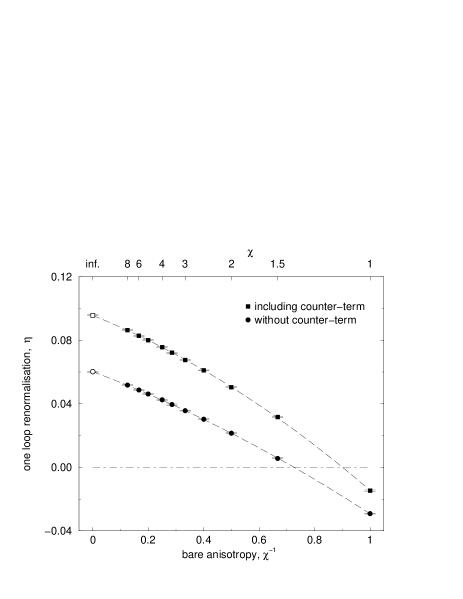
Figure 3: Anisotropy renormalisation for the spatially improved action as a function of the bare anisotropy $\chi$, showing fits quadratic in $\chi^{-1}$.

In both cases, the actual calculation proceeds as for the Wilson action (the only changes in the loop integration code being the Python–generated input files). In Fig. 3 we plot $\eta(\chi)$ as a function of $\chi$. The results are also presented in Table 1. The slightly larger errors in the full calculation reflects a greater uncertainty in the extrapolation in $L$ due to reduced data.

These values can be fitted extremely well, as is demonstrated in Fig. 3, by

$$\eta(\chi)=0.0602\;(1)-0.0656\;(2)\frac{1}{\chi}-0.0237\;(1)\frac{1}{\chi^{2}}$$ (100)

without the mean link counterterm contribution, and

$$\eta(\chi)=0.0955\;(4)-0.0702\;(16)\frac{1}{\chi}-0.0399\;(14)\frac{1}{\chi^{2}}$$ (101)

when this is included.

III.2 comparison with measured data

The goal of this paper is to provide determinations of the renormalied anisotropy using perturbation theory. It is clear that for sufficiently small couplings the one loop result will be sufficient, but at couplings more typical of current lattice simulations we must check what systematic truncation errors are introduced by neglecting contributions of higher orders. We can do this by comparing the perturbative predictions with what measurements have been made in Monte Carlo simulations.

We start with the Symanzik improved action, for which measurements of $\chi_{R}$ have been published in alea ; shigemitsu02 , derived from torelon dispersion relations and the so-called sideways potential.

We have obtained as a perturbative series, $Z(g^{2},\chi,v)=1+\eta(\chi,v)g^{2}+O(g^{4})$. Such a series, however, shows poor convergence and thus large truncation errors. We can re-express it as a power series in the ‘self-consistent’, or ‘boosted’ coupling, ${g_{0}}^{2}$:

$$Z({g_{0}}^{2},\chi)=1+\eta(\chi,v=u_{s}){g_{0}}^{2}+O({g_{0}}^{4})\;,$$ (102)

using the definitions in Eqn. (89). For appropriate choices of tadpole improvement schemes, the convergence is much improved. In resumming the series, we formally require only that $u_{s,t}$ are self-consistent for fixed $\beta_{0},\chi_{0}$ up to a suitable order of perturbation theory, and that $v=u_{s}$ to the same order. There are arguments, however, for satisfying these conditions at a numerical level for greater convergence. The one loop result is, of course, unchanged under resummation.

The action in alea ; shigemitsu02 contains explicit factors of $u_{s,t}$ and before applying $Z$ it is necessary to rescale $\chi_{0}$ to $\chi$ using the simulated values of the mean link factors. In Table 2 we compare the one loop perturbative determination with the published measurements. The couplings are larger than those used in many simulations (giving a relatively coarse spatial lattice), and the anisotropy factors are at the higher end of those usually employed, making this a rather stringent test of the perturbative series. Despite this, we find this error to be uniformly small. For $\chi_{0}\leq 4$ the error is 2%, and for $\chi_{0}=6$ it is only 3%. If we attribute the difference between the measured and one loop estimate to be that due to truncation of the perturbative series, it is clear that the two loop contribution to $Z$ is very small. The range of couplings, however, is insufficient to allow us to reliably estimate the two loop coefficient from the data.

A comparison of the one loop perturbative and measured anisotropy has been carried out for the Wilson action by Klassen klassen98 . Corroboration of this analysis is hampered by a lack of published tadpole improvement factors. Whilst $\chi$ is quoted directly, $u_{s,t}$ are required to obtain the self-consistent coupling, ${g_{0}}^{2}$, appropriate to simulated values of $\beta$. We may estimate the tadpole factors, but in doing so we introduce a second systematic error into the estimate of $\chi_{R}$. This arises from the difference between our estimate and the numerically self-consistent tadpole values. It is in addition to the systematic error arising from the one loop truncation of the perturbative expansion of $Z$. We anticipate the latter being of order 3%, and we thus require values of $u_{s,t}$ at least this accurate. Such an estimate can come from a two loop perturbative estimate lat02 ; meanlink02 . Using this we have confirmed using Landau mean link improvement Klassen’s analysis (which used plaquette tadpole factors). We find the combined two loop tadpole, one loop anisotropy prediction for $\chi_{R}$ to be correct to within 5% for $\beta\geq 5.6$, and to 2% for $\beta\geq 6.3$ for $1.5\leq\chi\leq 6$. With the correct $u_{s,t}$ values, a more precise estimate of the truncation errors in $Z(\chi,g^{2})$ would be possible, and we expect them to show that the one loop anisotropy renormalisation calculation is as accurate for the Wilson action as we have demonstrated it to be for the Symanzik improved case.

IV Summary

We have presented perturbative calculations of the renormalisation of the anisotropy in simple gluonic lattice actions for SU(3) in $D=3+1$. These have been carried out by studying the infrared dispersion relation of the on-shell gluonic propagator, regulated through the use of twisted boundary conditions as in luwe . We have reviewed the derivation of the Feynman rules for general actions and anisotropy structure, using both twisted and untwisted boundary conditions. We have (briefly) outlined our method for generating the gluon $r$-point vertex functions using a Python code and evaluating the loop integrals using a compiled programming language. The strength of this dual–pronged approach is the generality; at the price of not carrying out optimisation specific to a particular action, a flexibility to rapidly change actions is acquired. Further details of the implementation will be given in meanlink02 .

We have focussed our attention on two actions, the Wilson plaquette action and an action (Symanzik) improved at tree level through the addition of $1\times 2$ loops extending two lattice spacings in spatial directions only. This lack of symmetry is necessary to avoid spurious ghost poles in the gluonic propagator, and in consequence even an isotropic lattice will not remain so under quantum corrections. Temporal improvement is not crucial, of course, when $a_{t}$ is small.

Both actions are considered with and without tadpole improvement of the links. In the case of the Wilson action no explicit reference to $u_{s,t}$ need be made in the perturbation theory. Specific tadpole improvement schemes manifest only in rescaling the gauge coupling.

For the Symanzik improved action, the lack of temporal improvement means all reference to $u_{t}$ can be reparametrized away, but dependence on $u_{s}$ remains in the form of a counterterm to the (tadpole) unimproved action. The presence of the counterterm necessarily specialized the perturbative calculation to one form of tadpole improvement, and we selected self-consistent Landau gauge mean links for this work.

There are also advantages in using this reparametrization when tuning actions such as $S_{SI}$ for Monte Carlo simulation, when explicit tadpole factors $u_{s,t}$ are often present. reparametrizing to remove dependence on $u_{t}$ makes the finding of a self-consistent $u_{s}$ for fixed $(\beta,\chi)$ a one parameter problem. Similarly tuning $u_{t}$ is done by varying $(\beta_{0},\chi_{0},u_{t})$ together along the single parameter curve of constant $(\beta,\chi,u_{s})$. This two stage approach is much faster than a simultaneous exploration of the two parameter space.

For the Symanzik improved action, we presented results over a spread of bare anisotropies $1\leq\chi_{0}\leq 8$, and give interpolating fits, Eqns. (100, 101), respectively with and without (Landau) mean link tadpole improvement. Comparing these numbers with measurements in simulations shows that the one loop perturbative determinations of the renormalized anisotropy are accurate to within 2% for $\chi\leq 4$ across a range in couplings and lattice spacings much larger than would typically be used in lattice simulations. For $\chi=6$, which is larger than that currently employed in large scale simulations, the deviation is 3%.

In the case of the Wilson action we have verified existing results (calculated using the background field method) by Snippe snip and Pérez and van Baal peba . Using an interpolating fit, Eqn. (96), we have carried out a comparison with lattice simulation results by Klassen klassen98 . We find the agreement to be approximately 3–4% for gauge couplings in the typically simulated range and $\chi\leq 6$, but this uncertainty includes a systematic error from having to estimate tadpole improvement factors, and the error in the anisotropy alone is almost certainly less.

We conclude that the renormalisation of the anisotropy, which is difficult to calculate accurately in simulations, is well described by lattice perturbation theory. If the anisotropy is to be used, for instance, to set the scale in lattice calculations as per Eqn. (1), then a 3% systematic error in $\chi_{R}$ is sufficiently small that is unlikely to represent the dominant uncertainty in the final estimate, and the one loop determinations presented in this paper are all that is required.

	Wilson	Spatially Improved
$\chi$		(a)	(b)
1	0	$-0$.02907 (1)	$-0$.01461 (30)
1.5	-	0.005654 (5)	0.03163 (30)
2	0.085303 (1)	0.021446 (4)	0.05037 (30)
2.5	-	0.03027 (1)	0.06097 (30)
3	-	0.035692 (8)	0.06753 (30)
3.5	-	0.03955 (1)	0.07218 (30)
4	0.127901 (2)	0.04251 (1)	0.07567 (30)
5	-	0.04851 (2)	0.08000 (30)
6	-	0.04851 (2)	0.08279 (30)
8	-	0.05172 (5)	0.08637 (30)

Table 1: Anisotropy renormalisation, $\eta$, for various $\chi$ for Wilson and Symanzik improved actions. The latter is shown (a) without and (b) with the spatial mean link counterterm contribution of Fig. 1(f).

$\beta_{0}$	$\chi_{0}$	$u_{s}$	$u_{t}$	$a_{s}^{-1}$	$\chi_{R}^{\rm(meas.)}$	$\chi$	$\eta(\chi)$	$\chi_{R}^{\rm(pert.)}$
				(MeV)
1.7	4	0.7164	0.98295	661 (11)	3.56 (2)	2.915	0.0667	3.601
	6	0.7100	0.99158	779 (28)	5.28 (2)	4.296	0.0770	5.463
1.8	4	0.7279	0.98243	797 (21)	3.61 (2)	2.964	0.0673	3.629
	6	0.7216	0.99208	839 (9)	5.31 (2)	4.364	0.0773	5.489
2.4	3	0.7868	0.9771	1200 (50)	2.71 (3)	2.416	0.0596	2.776

Table 2: Renormalized anisotropy as determined from torelon dispersion relations and the sideways potential shigemitsu02 ; alea , and from one loop perturbation theory.

Figure 1: Self energy graphs at $O(g^{2})$ for the gluon propagator. Graph (f) arises from treating the spatial mean link factor as a counterterm, and has a coupling proportional to the one loop expression for this.

Figure 2: Anisotropy renormalisation for the Wilson action as a function of $L$ for bare anisotropy $\chi=2$.