Perturbative calculation of $O(a)$ improvement coefficients

Abstract

We compute several coefficients needed for $O(a)$ improvement of currents in perturbation theory, using the Brodsky-Lepage-Mackenzie prescription for choosing an optimal scale $q^{*}$. We then compare the results to non-perturbative calculations. Normalization factors of the vector and axial vector currents show good agreement, especially when allowing for small two-loop effects. On the other hand, there are large discrepancies in the coefficients of $O(a)$ improvement terms. We suspect that they arise primarily from power corrections inherent in the non-perturbative methods.

I Introduction

During the past few years the Symanzik effective field theory has been an important focus of research in lattice gauge theory. Symanzik’s idea is to describe cutoff effects in lattice field theory by a continuum effective field theory Symanzik:1979ph . One writes Symanzik:1979ph ; Symanzik:1983dc

$${\cal L}_{\text{lat}}\doteq{\cal L}_{\text{Sym}},$$ (1)

where the symbol $\doteq$ means that the lattice and Symanzik field theories have the same on-shell matrix elements. For lattice QCD with Wilson fermions Wilson:1975hf the Symanzik local effective Lagrangian (LE${\cal L}$) is given by Sheikholeslami:1985ij ; Kronfeld:2002pi

$${\cal L}_{\text{Sym}}=\frac{1}{2g^{2}}\mathop{\textrm{tr}}[F^{\mu\nu}F_{\mu\nu}]-\bar{q}\left({\kern 1.00006pt/\kern-6.49994ptD}+m\right)q+aK_{\sigma\cdot F}\,\bar{q}i\sigma_{\mu\nu}F^{\mu\nu}q+O(a^{2}),$$ (2)

where $g^{2}$ is a renormalized coupling, $m$ is a renormalized quark mass, and $aK_{\sigma\cdot F}$ is a short-distance coefficient. The effective field theory is useful when the scale of QCD in lattice units is small, $\Lambda a\ll 1$, and, as used in this paper, when $ma\ll 1$ also. With the description in hand, the lattice field theory can be adjusted so that it approaches its continuum limit more quickly. The effective theory shows that if $K_{\sigma\cdot F}$ is reduced for any given on-shell matrix element, then the $O(a)$ term in Eq. (2) makes commensurately smaller contributions to all other on-shell matrix elements. This application of the Symanzik effective field theory is called the Symanzik improvement program Symanzik:1983dc .

A similar correspondence is set up for the vector and axial vector currents (see below), introducing further short-distance coefficients. In the last several years methods have been devised to study all of them non-perturbatively Jansen:1996ck ; Luscher:1996sc ; Martinelli:1997zc ; deDivitiis:1997ka ; Bhattacharya:1999uq . The $O(a)$ discretization effects violate chiral symmetry, so the key idea is to ensure that violations of chiral symmetry are at least $O(a^{2})$. On the other hand, because of asymptotic freedom and the success of perturbative QCD, even at GeV energies Davier:1997kw , one expects perturbation theory to yield accurate estimates of the short-distance coefficients. In this paper, we compare a perturbative calculation of the currents’ short-distant coefficients to the non-perturbative results.

There are two issues that should be kept in mind when making such a comparison. First, the non-perturbative technique suffers from power corrections. Asymptotically, as $\Lambda a\to 0$ these are formally smaller than any error made from truncating the perturbation series. In practice, however, these effects can be significant.

Second, no two-loop results are available for the improvement coefficients considered here. Tests of perturbation theory are, therefore, not unambiguous, because different choices for the expansion parameter $g^{2}$ yield quantitatively different results. The bare coupling $g_{0}^{2}$ (for the Wilson gauge action) is an especially bad expansion parameter Lepage1991:zt . The obvious remedy is to rearrange the perturbative series, eliminating $g_{0}^{2}$ in favor of a renormalized (running) coupling, evaluated at a scale characteristic of the problem at hand. One is then faced, however, with many choices of renormalization scheme, and the question of how to determine the “characteristic scale.” In this paper we choose the Brodsky-Lepage-Mackenzie (BLM) prescription Brodsky:1983gc ; Lepage:1993xa . Once this choice is made, little subjectivity remains, so one can ask quantitatively whether one-loop BLM perturbation theory agrees with the non-perturbative method.

In the BLM method, the characteristic scale is computed from Feynman diagrams. The new information presented in this paper consists of the calculations needed to determine the BLM scales of the normalization and improvement coefficients of the vector and axial vector currents for Wilson fermions with Sheikholeslami-Wohlert action. These calculations are a by-product of our recent work on the normalization and improvement of lattice currents with heavy quarks Harada:2001fi . Details of the calculational method may be found there.

This paper is organized as follows. In Sec. II we define the lattice currents and review their description in the Symanzik effective field theory. Section III recalls the BLM prescription, focusing on points that are sometimes overlooked. Our new results for the BLM scales are given in Sec. IV. This paves the way for a systematic comparison with non-perturbative calculations of the same quantities in Sec. V. Section VI contains a few concluding remarks.

II Lattice Currents

In this section we review the description of lattice currents with the Symanzik effective field theory. For quarks we take the Sheikholeslami-Wohlert Lagrangian Sheikholeslami:1985ij , which has an improvement coupling $c_{\text{SW}}$. At the tree level $K_{\sigma\cdot F}^{[0]}=\frac{1}{4}(1-c_{\text{SW}})$, so the improvement condition $K_{\sigma\cdot F}=0$ requires $c_{\text{SW}}=1+O(g^{2})$. For one-loop calculations, it is sufficient to specify $c_{\text{SW}}$ at the tree level. For the non-perturbative calculations cited below, $c_{\text{SW}}-1$ is determined non-perturbatively by the methods of Ref. Luscher:1996sc .

We denote the lattice fermion field with $\psi$. The lattice vector and axial vector currents take the form

$$V^{\mu}_{\text{lat}} = \bar{\psi}i\gamma^{\mu}\psi-ac_{V}{\partial_{\nu}}_{\text{lat}}\bar{\psi}\sigma^{\mu\nu}\psi,$$ (3)

$$A^{\mu}_{\text{lat}} = \bar{\psi}i\gamma^{\mu}\gamma_{5}\psi+ac_{A}\partial^{\mu}_{\text{lat}}\bar{\psi}i\gamma_{5}\psi.$$ (4)

The improvement couplings $c_{V}$ and $c_{A}$ should be chosen to reduce lattice artifacts, as discussed below. In Symanzik’s theory of cutoff effects, the lattice currents are described by operators in a continuum effective field theory Symanzik:1979ph ; Symanzik:1983dc ; Kronfeld:2002pi ; Luscher:1996sc

$$V^{\mu}_{\text{lat}} \doteq \bar{Z}_{V}^{-1}\bar{q}i\gamma^{\mu}q-aK_{V}\partial_{\nu}\bar{q}\sigma^{\mu\nu}q+\cdots,$$ (5)

$$A^{\mu}_{\text{lat}} \doteq \bar{Z}_{A}^{-1}\bar{q}i\gamma^{\mu}\gamma_{5}q+aK_{A}\partial^{\mu}\bar{q}i\gamma_{5}q+\cdots,$$ (6)

where, as in Eq. (2), $q$ is a continuum fermion field whose dynamics is defined by ${\cal L}_{\text{QCD}}$. The ellipsis indicates operators of dimension five and higher. Further dimension-four operators are omitted from Eqs. (5) and (6), because they are linear combinations of those listed and others that vanish by the equations of motion. The short-distance coefficients in the effective Lagrangian—$\bar{Z}_{J}$ and $K_{J}$ ($J=V$, $A$)—are functions of $g^{2}$ and $ma$, and the improvement couplings $c_{\text{SW}}$ and $c_{J}$.

Symanzik improvement is achieved by adjusting $c_{J}$ so that $K_{J}=0$. Then $\bar{Z}_{V}V^{\mu}_{\text{lat}}$ and $\bar{Z}_{A}A^{\mu}_{\text{lat}}$ have the same matrix elements as $\bar{q}i\gamma^{\mu}q$ and $\bar{q}i\gamma^{\mu}\gamma_{5}q$, apart from lattice artifacts of order $a^{2}$. For light quarks one may expand $\bar{Z}_{J}$ in $ma$,

$$\bar{Z}_{J}=Z_{J}\left(1+mab_{J}\right),$$ (7)

and identify $K_{J}$ with the zeroth order of a small $ma$ expansion. At the tree level the coefficients of the normalization factor are $Z_{J}^{[0]}=1$, $b_{J}^{[0]}=1$. In addition, the coefficient of the lattice artifact is

$$K_{J}^{[0]}=c_{J}^{[0]}.$$ (8)

The improvement condition $K_{J}=0$ says that one should set $c_{J}^{[0]}=0$. Consequently, one-loop calculations are based solely on the first terms in Eqs. (3) and (4).

III Brodsky-Lepage-Mackenzie Prescription

In this section we review the BLM prescription, following the argumentation from Ref. Lepage:1993xa . This material should be familiar, but some of the literature on non-perturbative improvement blurs the difference between BLM perturbation theory and other topics, such as “tadpole improvement” and mean-field estimates of the renormalized coupling, which are also discussed in Ref. Lepage:1993xa .

The problem is to find a reasonably accurate one-loop estimate of a quantity $\zeta$, here $\bar{Z}_{J}$ or $K_{J}$. In these cases, one gluon with momentum $k$ and propagator $D(k)$ appears. The contribution from the Feynman diagrams can be written

$$g^{2}_{R}\zeta^{[1]}(p)=g_{0}^{2}\int\frac{d^{4}k}{(2\pi)^{4}}D(k)f(k,p)+\cdots,$$ (9)

where $p$ denotes $k$-independent parameters, such as external momenta. The ellipsis indicates higher-order terms that we would like to absorb into the renormalized coupling $g^{2}_{R}$. An important class of higher-order terms consists of the renormalization parts that dress the exchanged gluon. In the Fourier transform of the heavy-quark potential, for example, they turn $g_{0}^{2}D(k)$ into $g_{V}^{2}(k)D(k)$, where the potential $V(q)=-C_{F}g^{2}_{V}(q)/q^{2}$. Thus,

$$g^{2}_{R}\zeta^{[1]}(p)=\int\frac{d^{4}k}{(2\pi)^{4}}g_{V}^{2}(k)D(k)f(k,p)+\cdots$$ (10)

sums the renormalization parts. Other ways of dressing the gluon would lead to other physical running couplings, but they all are the same at order $\beta_{0}g^{4}$ Brodsky:1983gc , where $\beta_{0}=11-\frac{2}{3}n_{f}$ is the one-loop coefficient of the $\beta$ function for $n_{f}$ light quarks.

If there is a characteristic scale $q^{*}$, one can approximate

$$g_{V}^{2}(k) = \frac{g_{V}^{2}(q^{*})}{1+(\beta_{0}/16\pi^{2})g_{V}^{2}(q^{*})\ln(k/q^{*})^{2}}$$ (11)

$$= g_{V}^{2}(q^{*})+\frac{\beta_{0}}{16\pi^{2}}g_{V}^{4}(q^{*})\ln(q^{*}/k)^{2}+\cdots.$$ (12)

The aim is to choose $q^{*}$ so that higher-order terms are small, particularly those of order $\beta_{0}g_{V}^{4}$, which could be enhanced by a foolish choice of $q^{*}$. Inserting Eq. (12) into Eq. (10) and setting the coefficient of $\beta_{0}g_{V}^{4}$ to zero yields

$$\ln q^{*}a=\frac{{}^{*}\zeta^{[1]}}{2\zeta^{[1]}},$$ (13)

where $a$ is a reference short-distance scale (namely, the lattice spacing), and

$${}^{*}\zeta^{[1]}(p)=\int\frac{d^{4}k}{(2\pi)^{4}}\ln(ka)^{2}D(k)f(k,p).$$ (14)

Thus, the BLM prescription is to set $g_{R}^{2}=g_{V}^{2}(q^{*})$ in the one-loop approximation.

If one prefers a different renormalized coupling, one must change the scale in the appropriate way. The coupling in scheme “$S$” is related to the $V$ scheme by

$$\frac{1}{g^{2}_{S}(q)}=\frac{1}{g^{2}_{V}(q)}+\frac{\beta_{0}b_{S}^{(1)}+b_{S}^{(0)}}{16\pi^{2}}+O(g^{2}),$$ (15)

where $b_{S}^{(0)}$ and $b_{S}^{(1)}$ are constants independent of $n_{f}$. The BLM scale $q^{*}_{S}$ for this scheme is given by

$$\ln q^{*}_{S}=\ln q^{*}-\frac{1}{2}b_{S}^{(1)}.$$ (16)

For example, for the modified minimal subtraction ($\overline{\rm MS}$) scheme, $b_{\overline{\rm MS}}^{(0)}=-8$ and $b_{\overline{\rm MS}}^{(1)}=5/3$, $q^{*}_{\overline{\rm MS}}=e^{-5/6}q^{*}=0.435q^{*}$. With Eq. (16) one recovers the summary statement of Ref. Brodsky:1983gc , namely to absorb into $q^{*}_{S}$ the $n_{f}$ dependence of the two-loop term, which enters through $\beta_{0}$.

The BLM prescription has several features that make it a natural choice in matching calculations, such as those considered in this paper. The effective field theory framework suggests using a renormalized coupling, in particular one that has a (quasi-)physical definition in both the underlying theory (here lattice gauge theory) and in the effective theory (here the Symanzik effective field theory). For quantitative purposes it is more interesting to note that

$$\frac{1}{g^{2}_{S}(q^{*}_{S})}=\frac{1}{g^{2}_{V}(q^{*})}+\frac{b_{S}^{(0)}}{16\pi^{2}}+O(g^{2}),$$ (17)

so the numerical difference in the BLM expansion parameters is small, as long as $g^{2}b_{S}^{(0)}/16\pi^{2}$ is small.

IV Perturbative Results

In Ref. Harada:2001fi we found for gauge group SU(3) and $c_{\text{SW}}=1$

$$Z_{V}^{[1]} = -0.129423(6),$$ (18)

$$Z_{A}^{[1]} = -0.116450(5),$$ (19)

in excellent agreement with previous work Gabrielli:1990us ; Capitani:2001xi . (Reference Capitani:2001xi gives precise results as a polynomial in $c_{\text{SW}}$.) We also found (with $c_{J}^{[0]}=0$)

$$b_{V}^{[1]} = 0.153239(14),$$ (20)

$$b_{A}^{[1]} = 0.152189(14),$$ (21)

$$K_{V}^{[1]} = c_{V}^{[1]}+0.016332(7),$$ (22)

$$K_{A}^{[1]} = c_{A}^{[1]}+0.0075741(15),$$ (23)

which agree perfectly with Ref. Sint:1997jx . Solving the improvement condition $K_{J}=0$ at this order gives

$$c_{V}^{[1]} = -0.016332(7),$$ (24)

$$c_{A}^{[1]} = -0.0075741(15).$$ (25)

We also directly obtained

$$b_{V}^{[1]}-b_{A}^{[1]}=0.0010444(16),$$ (26)

which is more accurate than the difference of the two numbers quoted above. In taking the difference, large contributions from the self energy cancel, but, even so, the near equality of $b_{V}^{[1]}$ and $b_{A}^{[1]}$ is a bit astonishing. The mass dependence of $\bar{Z}_{J}$ shows that $b_{V}^{[1]}-b_{A}^{[1]}$ is not so small for the Wilson action Harada:2001fi .

In our method for computing the improvement coefficients it is easy to weight the integrands with $\ln(ka)^{2}$ and, thus, obtain the BLM scales. We find

$${}^{*}Z_{V}^{[1]} = -0.270691(19),$$ (27)

$${}^{*}Z_{A}^{[1]} = -0.243086(09),$$ (28)

$${}^{*}b_{V}^{[1]} = 0.321556(35),$$ (29)

$${}^{*}b_{A}^{[1]} = 0.318108(21),$$ (30)

$${}^{*}b_{V}^{[1]}-{}^{*}b_{A}^{[1]} = 0.0034247(51),$$ (31)

$${}^{*}c_{V}^{[1]} = -0.0222383(15),$$ (32)

$${}^{*}c_{A}^{[1]} = -0.0147825(62),$$ (33)

and hence

$$q^{*}_{Z_{V}}a = 2.846,$$ (34)

$$q^{*}_{Z_{A}}a = 2.840,$$ (35)

$$q^{*}_{Z_{A}/Z_{V}}a = 2.898,$$ (36)

$$q^{*}_{b_{V}}a = 2.855,$$ (37)

$$q^{*}_{b_{A}}a = 2.844,$$ (38)

$$q^{*}_{b_{V}-b_{A}}a = 5.153,$$ (39)

$$q^{*}_{c_{V}}a = 1.975,$$ (40)

$$q^{*}_{c_{A}}a = 2.653.$$ (41)

The scales are in the expected range. The higher scale for $b_{V}-b_{A}$ means simply that the difference between these renormalization constants arises from very short distances. These numerical results are new; they have been obtained from two independent computer programs. As a further check, we have reproduced the values of $q^{*}_{Z_{V}}a$ and $q^{*}_{Z_{A}}a$ for the Wilson action ($c_{\text{SW}}=0$), given in Ref. Bernard:1998sx .

The dominant contributor to the “large” one-loop normalization constants, Eqs. (18)–(21), is the tadpole diagram (in Feynman gauge) of the self energy. One might expect perturbation theory to work better for quantities in which the effects of tadpole diagrams largely cancel (albeit in a gauge-invariant way). For example, $Z_{A}/Z_{V}$ and $b_{V}-b_{A}$ are tadpole free and have smaller one-loop coefficients.

Another way to remove the tadpoles is to write

$$Z_{J}=u_{0}\tilde{Z}_{J},$$ (42)

$$b_{J}=\tilde{b}_{J}/u_{0},$$ (43)

where $u_{0}$ is any convenient tadpole-dominated quantity. Then one can take $u_{0}$ from a non-perturbative Monte Carlo calculation and use perturbation theory for $\tilde{Z}_{J}$ and $\tilde{b}_{J}$. The corresponding one-loop coefficients are

$$\tilde{Z}_{J}^{[1]}=Z_{J}^{[1]}-u_{0}^{[1]},$$ (44)

$$\tilde{b}_{J}^{[1]}=b_{J}^{[1]}+u_{0}^{[1]}.$$ (45)

Similarly, to get the BLM scale

$${}^{*}\tilde{Z}_{J}^{[1]}={}^{*}Z_{J}^{[1]}-{}^{*}u_{0}^{[1]},$$ (46)

$${}^{*}\tilde{b}_{J}^{[1]}={}^{*}b_{J}^{[1]}+{}^{*}u_{0}^{[1]},$$ (47)

where ${}^{*}u_{0}^{[1]}$ is the BLM numerator [cf. Eq. (13)] for $u_{0}$. Below we take $u_{0}^{4}$ to be the average value of the plaquette, with $u_{0}^{[1]}=-1/12=-0.08\bar{3}$ and ${}^{*}u_{0}^{[1]}=-0.204049(1)$. A glance at Eqs. (44)–(47) shows immediately that tadpole improvement reduces the one-loop coefficients. With tadpole improvement the BLM scales become

$$q^{*}_{\tilde{Z}_{V}}a = 2.061,$$ (48)

$$q^{*}_{\tilde{Z}_{A}}a = 1.803,$$ (49)

$$q^{*}_{\tilde{b}_{V}}a = 2.317,$$ (50)

$$q^{*}_{\tilde{b}_{A}}a = 2.289.$$ (51)

The scales are lower than without tadpole improvement, but still ultraviolet.

It is perhaps worthwhile emphasizing the difference between tadpole improvement and the BLM prescription. The aim of tadpole improvement is to re-sum large contributions appearing at order $g^{2}$ and higher, replacing the sum with a non-perturbative estimate ($u_{0}$, for example). The aim of the BLM prescription is to re-sum potentially large renormalization parts into the renormalized coupling. Although the aims are similar, they are not identical. They are not mutually exclusive, and neither is a substitute for the other.

V Comparison to Non-perturbative Calculations

Table 1: Comparison of perturbative and non-perturbative determinations of the improvement coefficients at $\beta=6.2$.

$\beta=6.2$	$\alpha_{V}(q^{*})$	BLM	Refs. Luscher:1996ck ; Luscher:1996ax ; Guagnelli:1997db	Ref. Bhattacharya:2001pn
$Z_{V}$	0.1468	0.7612	0.7922(9)	0.7874(4)
$Z_{A}$	0.1469	0.7850	0.807(8)	0.818(5)
$Z_{A}/Z_{V}$	0.1461	1.0238	1.019(8)	1.039(5)
$b_{V}$	0.1467	1.2824	1.41(2)	1.42(1)
$b_{A}$	0.1468	1.2808	—	1.32(5)
$b_{V}-b_{A}$	0.1257	0.001649	—	0.11(5)
$-c_{V}$	0.1638	0.03361	0.21(7)	0.09(2)
$-c_{A}$	0.1498	0.01426	0.038(4)	0.032(7)
$u_{0}\tilde{Z}_{V}$	0.1616	0.8022	0.7922(9)	0.7874(4)
$u_{0}\tilde{Z}_{A}$	0.1686	0.8230	0.807(8)	0.818(5)
$\tilde{b}_{V}/u_{0}$	0.1559	1.2846	1.41(2)	1.42(1)
$\tilde{b}_{A}/u_{0}$	0.1565	1.2828	—	1.32(5)

Table 2: Comparison of perturbative and non-perturbative determinations of the improvement coefficients at $\beta=6.0$.

$\beta=6.0$	$\alpha_{V}(q^{*})$	BLM	Refs. Luscher:1996ck ; Luscher:1996ax ; Guagnelli:1997db	Ref. Bhattacharya:2001pn
$Z_{V}$	0.1602	0.7394	0.7809(6)	0.770(1)
$Z_{A}$	0.1603	0.7654	0.791(9)	0.807(8)
$Z_{A}/Z_{V}$	0.1593	1.0260	1.012(9)	1.048(8)
$b_{V}$	0.1601	1.3082	1.54(2)	1.52(1)
$b_{A}$	0.1603	1.3065	—	1.28(5)
$b_{V}-b_{A}$	0.1352	0.001774	—	0.24(5)
$-c_{V}$	0.1808	0.03711	0.32(7)	0.107(17)
$-c_{A}$	0.1638	0.01559	0.083(5)	0.037(9)
$u_{0}\tilde{Z}_{V}$	0.1782	0.7872	0.7809(6)	0.770(1)
$u_{0}\tilde{Z}_{A}$	0.1868	0.8095	0.791(9)	0.807(8)
$\tilde{b}_{V}/u_{0}$	0.1712	1.3105	1.54(2)	1.52(1)
$\tilde{b}_{A}/u_{0}$	0.1719	1.3087	—	1.28(5)

With the BLM scales in hand we can compare the prediction of one-loop BLM-improved perturbation theory with non-perturbative determinations of the improvement coefficients. We shall make the comparison in two ways. First we compare the numerical values directly, at two values of the bare coupling. Here there are two methods in the literature, one based on finite-size techniques and the Schrödinger functional Luscher:1996ck ; Luscher:1996ax ; Guagnelli:1997db , and another based on large volumes with hadronic matrix elements Bhattacharya:2001pn . The difference between these two illustrates how large power corrections to the improvement coefficients are. We also compare our results graphically, as a function of coupling, to Padé approximants given in Refs. Sint:1997jx ; Luscher:1996ck ; Luscher:1996ax . These graphs are helpful for seeing whether discrepancies in the one-loop and non-perturbative estimates arise from two-loop or power corrections.

We obtain $\alpha_{V}(q^{*})$ as follows. First we compute

$$\alpha_{1\times 1}=-\frac{3}{4\pi}\ln\langle\Box\rangle,$$ (52)

where $\langle\Box\rangle$ is the ensemble average of the plaquette. Then we follow Ref. Lepage:1993xa and take $\alpha_{V}$ to be

$$\alpha_{V}(3.402/a)\equiv\frac{2\alpha_{1\times 1}}{1+\sqrt{1-4.741\alpha_{1\times 1}}},$$ (53)

which agrees with the standard definition of $\alpha_{V}$ with an accuracy of order $\alpha_{s}^{3}$. The scale $3.402/a$ is the BLM scale for $\langle\Box\rangle$. We then run from $3.402/a$ to $q^{*}$ with the two-loop evolution equation. Of course, once two-loop perturbation theory is available, one would have to extend the accuracy of Eq. (53) and of the evolution.

Table 1 gives results from our perturbative calculation with non-perturbative results from the Alpha Collaboration Luscher:1996ck ; Luscher:1996ax ; Guagnelli:1997db and from Bhattacharya et al. Bhattacharya:2001pn , at $\beta=6.2$. Table 2 gives the same comparison at $\beta=6.0$. Above (below) the horizontal line, we have applied the BLM prescription without (with) tadpole improvement. The error bars on the entries from Refs. Luscher:1996ck ; Luscher:1996ax ; Guagnelli:1997db ; Bhattacharya:2001pn are statistical, and compiled in Ref. Bhattacharya:2001pn .

For the normalization factors $Z_{V}$ and $Z_{A}$, BLM perturbation theory and the non-perturbative methods agree well, within 3–4%. The difference between the two non-perturbative values of $Z_{V}$ exceeds the reported errors, but is easily explained by power correction of order $(\Lambda a)^{2}$. For the tadpole-free ratio $Z_{A}/Z_{V}$ and for the tadpole-improved quantities $u_{0}\tilde{Z}_{J}$, BLM perturbation theory lies very close to the non-perturbative range. These impressions are strengthened by Fig. 1, which shows $Z_{V}$ and $Z_{A}$ as functions of $g_{0}^{2}$.

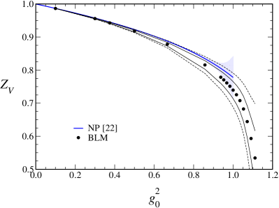
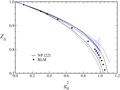
(a) (b)
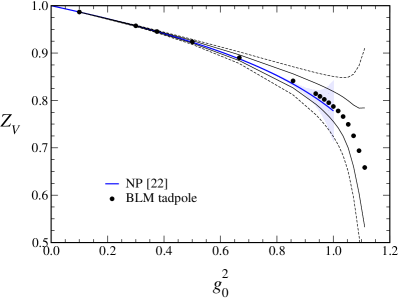
(c) (d)

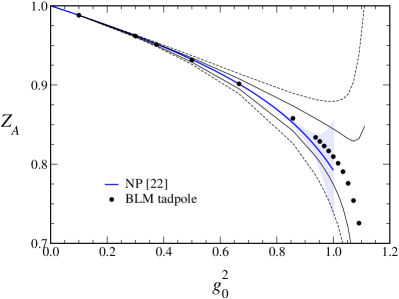
Figure 1: $Z_{V}$ and $Z_{A}$ vs. $g_{0}^{2}$. Heavy lines show the non-perturbative results, Eqs. (54) and (55), and shading possible corrections of order $\pm(\Lambda a)^{2}$. Circles show BLM perturbation theory, with thin and dashed lines to indicate a two-loop term $\pm\alpha_{V}^{2}$ or $\pm 2\alpha_{V}^{2}$. (a) and (c) no tadpole improvement, $Z_{J}^{\text{BLM}}=1+g_{V}^{2}(q^{*}_{Z_{J}})Z_{J}^{[1]}$; (b) and (d) with tadpole improvement, $Z_{J}^{\text{BLM}}=u_{0}[1+g_{V}^{2}(q^{*}_{\tilde{Z}_{J}})\tilde{Z}_{J}^{[1]}]$.

Circles show BLM perturbation theory, and the thin solid (dashed) lines indicate how two-loop contributions of $\pm\alpha_{V}^{2}$ ($\pm 2\alpha_{V}^{2}$) could modify the result. We show the result with and without tadpole improvement in Figs. 1(b,d) and (a,c), respectively. For the non-perturbative method, a heavy (blue) line shows the Padé approximants Luscher:1996ax

$$Z_{V} = \frac{1-0.7663g_{0}^{2}+0.0488g_{0}^{4}}{1-0.6369g_{0}^{2}},$$ (54)

$$Z_{A} = \frac{1-0.8496g_{0}^{2}+0.0610g_{0}^{4}}{1-0.7332g_{0}^{2}},$$ (55)

which deviate from the underlying calculations negligibly for $g_{0}^{2}\leq 1$. The shaded bands behind the Padé curves show a power-correction of $\pm(\Lambda a)^{2}$, with $\Lambda\sim 500~{}\textrm{GeV}$. The finite-volume result also suffers from power corrections of order $(a/L)^{2}$. They are estimated to be small by comparing calculations on lattices with $a/L=1/8$ and $1/12$ Luscher:1996ax . Also, they are parametrically smaller, because Ref. Luscher:1996ax holds $L\Lambda\sim 2$ for all $g_{0}^{2}$.

Next let us turn to the $O(ma)$ corrections to the normalization factors, $b_{V}$ and $b_{A}$. There is only one calculation of $b_{A}$ Bhattacharya:2001pn , so let us concentrate first on $b_{V}$. The two non-perturbative results for $b_{V}$ agree perfectly with each other (see the Tables), but they deviate significantly from one-loop BLM perturbation theory. Some insight can be gleaned from Fig. 2, which shows $b_{V}$ as a function of $g_{0}^{2}$.

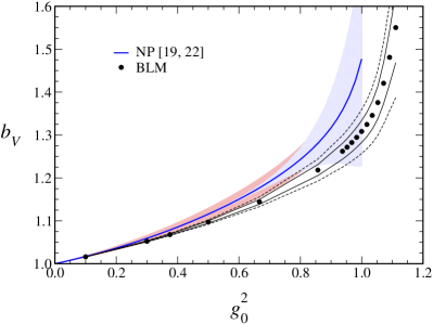
(a) (b)

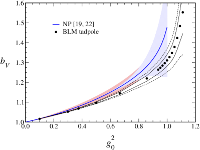
Figure 2: $b_{V}$ vs. $g_{0}^{2}$. (a) no tadpole improvement, $b_{V}^{\text{BLM}}=1+g_{V}^{2}(q^{*}_{b_{V}})b_{V}^{[1]}$; (b) with tadpole improvement, $b_{V}^{\text{BLM}}=[1+g_{V}^{2}(q^{*}_{\tilde{b}_{V}})\tilde{b}_{V}^{[1]}]/u_{0}$. Light grey (light blue) shading indicates power corrections to $b_{V}$ of order $\pm\Lambda a$; darker grey (pink) shading power corrections to $b_{V}-1$ of order $\pm a/L$.

The non-perturbative method is represented with the Padé approximant Sint:1997jx

$$b_{V}=\frac{1-0.7613g_{0}^{2}+0.0012g_{0}^{4}-0.1136g_{0}^{6}}{1-0.9145g_{0}^{2}},$$ (56)

with light (blue) shading for a power correction $\pm\Lambda a$. In finite volume there is also a power correction to $b_{V}$ of order $a/L$; by construction it applies to $b_{V}-1$ Luscher:1996ax , but now $L$ with $a$ varies such that $a/L=1/8$ for all $g_{0}^{2}$. We model this effect as $(b_{V}-1)(1\pm\frac{1}{8})$, shown in the darker (pink) shading in Fig. 2. Judging from its size and shape, the deviation seen in Fig. 2 looks less like a two-loop effect than a combination of power corrections of order $a/L$ and $\Lambda a$. (Similar conclusions are reached in Ref. Bhattacharya:2001pn .) There is almost no difference whether one applies tadpole improvement to $b_{V}$ or not, once the BLM prescription is applied. These two approximations truncate higher orders of the perturbation series differently, substantiating the idea that the discrepancy is a power correction.

The non-perturbative calculation of $b_{A}$ agrees with one-loop BLM perturbation theory. Note, however, that Ref. Bhattacharya:2001pn obtains $b_{V}$ and $b_{V}-b_{A}$ directly, and then $b_{A}=b_{V}-(b_{V}-b_{A})$. The agreement between BLM perturbation theory and the non-perturbative results for $b_{V}$ and $b_{V}-b_{A}$ is not good, so the agreement for $b_{A}$ may be an accident. Since the coefficient $b_{V}^{[1]}-b_{A}^{[1]}$ in Eq. (26) is remarkably small, the two-loop contribution could be as large as the one-loop term. Furthermore, inspection of Fig. 14 in Ref. Bhattacharya:2001pn suggests that a fit to the three smallest masses would yield a smaller value of $b_{V}-b_{A}$. We consider the comparison of $b_{A}$ and $b_{V}-b_{A}$ to be unsettled pending a two-loop calculation and a more robust non-perturbative calculation.

In any case, the mild disagreement on $b_{V}$ and $b_{V}-b_{A}$ is not of much practical importance. For the sake of argument, suppose $ma<0.1$, which holds for the light quarks for which the currents were designed. Then power corrections in $b_{J}$, at fixed $a$, lead to an uncertainty in a decay constant or a form factor of only a few per cent. After a continuum limit extrapolation, these uncertainties will not be important.

Now let us turn to the coefficients $c_{J}$ of the improvement terms in Eq. (3) and (4). At the tabulated values of $\beta$, the non-perturbative and BLM calculations of $c_{A}$ do not agree at all. At $\beta=6.0$ (Table 2) the two non-perturbative calculations also do not agree with each other. Figure 3(a) shows $c_{A}$ as a function of $g_{0}^{2}$,

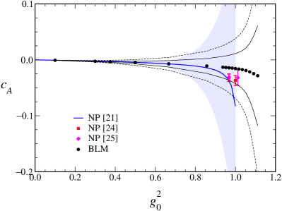
(a) (b)

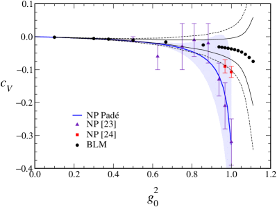
Figure 3: $c_{A}$ and $c_{V}$ vs. $g_{0}^{2}$. Shading shows power corrections of order $\pm\Lambda a$ to (a) Eq. (57), (b) Eq. (58). Points with error bars are from (a) Refs. Bhattacharya:2001pn ; Collins:2001mm , (b) Refs. Guagnelli:1997db ; Bhattacharya:2001pn .

using the Padé approximant Luscher:1996ck

$$c_{A}=-0.00756g_{0}^{2}\frac{1-0.748g_{0}^{2}}{1-0.977g_{0}^{2}}$$ (57)

to represent the non-perturbative calculations. The disagreement between BLM perturbation theory and Eq. (57) sets in for $g_{0}^{2}>0.9$. There are two reasons to suspect that the discrepancy stems from a power correction of order $\Lambda a$ to the results of Ref. Luscher:1996ck . First, Fig. 3(a) shows that it has the shape and size of such a power correction. Second, the extracted value of $c_{A}$ depends on the lattice derivative used to define the current Collins:2001mm . Note Bhattacharya:2001pn that errors in $c_{A}$ propagate to $c_{V}$, because in the Ward identities $c_{A}$ is multiplied by large hadronic matrix elements such as $am^{2}_{K}/m_{s}\sim a\times 2.5~{}\textrm{GeV}$. This enhancement also explains why Eq. (57) leads to worse scaling in $f_{\pi}$ Collins:2001mm . Figure 3(a) also includes the non-perturbative results of Refs. Bhattacharya:2001pn ; Collins:2001mm . The difference between those points and BLM perturbation theory could be a modest two-loop effect or a small power correction.

For $c_{V}$, the two non-perturbative results agree neither with each other, nor with BLM perturbation theory. The Alpha Collaboration has only a preliminary calculation Guagnelli:1997db . We have taken the liberty of extracting results from Fig. 3 of Ref. Guagnelli:1997db and fitting them to a Padé formula. The leading behavior is fixed to Eq. (24), and we obtain

$$c_{V}=-0.01633g_{0}^{2}\frac{1-0.257g_{0}^{2}}{1-0.963g_{0}^{2}}.$$ (58)

Figure 3(b) plots Eq. (58), the underlying points Guagnelli:1997db , the non-perturbative results from hadronic correlation functions Bhattacharya:2001pn , and BLM perturbation theory. As usual we show possible power corrections to Eq. (58) of order $\pm\Lambda a$, as well as the size of typical two-loop effects. At small $g_{0}^{2}$, there is good agreement with (BLM) perturbation theory, but once $g_{0}^{2}>0.9$, there is a sharp turnover. It is probably a power correction, possibly exacerbated by power corrections to $c_{A}$ as modeled by Eq. (57). With hadronic correlation functions Bhattacharya:2001pn the non-perturbative value of $c_{V}$ is half or a third as large. It is not clear at present whether the discrepancy between Ref. Bhattacharya:2001pn and BLM perturbation theory is a power correction to the former or a sizable two-loop correction to the latter.

We should also mention that BLM perturbation theory works better than several forms of mean-field perturbation theory (let alone bare perturbation theory). In Table 3 we list several choices for $\alpha_{s}$:

$$\alpha_{0}=g_{0}^{2}/4\pi,$$ (59)

$$\tilde{\alpha}_{0}=\alpha_{0}/u_{0},$$ (60)

as well as $\alpha_{1\times 1}$ [Eq. (52)] and $\alpha_{\overline{\rm MS}}(q^{*}_{\overline{\rm MS}})$ [Eq. (17)]. With only one-loop expansions available, the mean-field choices $\tilde{\alpha}_{0}$ and $\alpha_{1\times 1}$ give smaller corrections, and one-loop perturbation theory falls short even when power corrections are negligible. The consistency of BLM-$V$ perturbation theory for $Z_{V}$, $Z_{A}$, and $Z_{A}/Z_{V}$ indicates that the BLM prescription does indeed re-sum an important class of higher-order contributions. On the other hand, the coupling $\alpha_{\overline{\rm MS}}(q^{*}_{\overline{\rm MS}})$ seems, empirically, to work less well. In continuum perturbative QCD, it usually does not matter whether one adopts $\alpha_{V}(q^{*}_{V})$, $\alpha_{\overline{\rm MS}}(q^{*}_{\overline{\rm MS}})$ or some other renormalized coupling (at the BLM scale), once two-loop effects are included. It would not be surprising for the same to hold for short-distance quantities in lattice gauge theory, such as improvement coefficients.

Table 3: Expansion parameters for perturbation theory.

$\beta$	$\alpha_{0}$	$\tilde{\alpha}_{0}$	$\alpha_{1\times 1}$	$\alpha_{V}(q^{*}_{Z_{V}})$	$\alpha_{\overline{\rm MS}}(q^{*}_{Z_{V}})$
6.0	0.0796	0.1340	0.1245	0.1602	0.1784
6.2	0.0770	0.1255	0.1166	0.1468	0.1619
6.4	0.0746	0.1183	0.1101	0.1362	0.1491
7.0	0.0682	0.1016	0.0951	0.1134	0.1222
9.0	0.0531	0.0702	0.0667	0.0748	0.0786

VI Conclusions

In this paper we have compared non-perturbative calculations of several improvement coefficients to perturbation theory with the BLM prescription. Previously this could not be done, because the “BLM numerators” in Eqs. (27)–(33) were not available. We find that, for the scale-independent quantities considered here, the integration of the $\log k^{2}$-weighted integrals is numerically straightforward.

BLM perturbation theory for the current normalization factors $Z_{J}$ agrees very well with non-perturbative calculations of the same quantities. Here the leading power correction is only of order $(\Lambda a)^{2}$, and the small deviations can probably be removed with a two-loop calculation. Note that generalizations of the BLM method for higher-order perturbation theory have been considered in continuum perturbative QCD Brodsky:1994eh and in lattice gauge theory Hornbostel:2000ey .

For the improvement coefficients $b_{J}$ and $c_{J}$, the leading power corrections are of order $\Lambda a$ (and in the Schrödinger functional also of order $a/L=1/8$), while some of the one-loop coefficients are small. It is consequently difficult to diagnose the discrepancies. By noting the size and dependence on $g_{0}^{2}$ of the differences, we concur with the authors of Refs. Bhattacharya:2001pn ; Collins:2001mm , namely, that power corrections contaminate the non-perturbative results. In particular, it seems unlikely that higher orders in perturbative series could explain all discrepancies between one-loop BLM perturbation theory and the results from Refs. Luscher:1996ck ; Luscher:1996ax ; Guagnelli:1997db .

References

- (1) K. Symanzik, in Recent Developments in Gauge Theories, edited by G. ’t Hooft et al. (Plenum, New York, 1980).
- (2) K. Symanzik, in Mathematical Problems in Theoretical Physics, edited by R. Schrader et al. (Springer, New York, 1982); Nucl. Phys. B 226, 187, 205 (1983).
- (3) K. G. Wilson, in New Phenomena in Subnuclear Physics, edited by A. Zichichi (Plenum, New York, 1977).
- (4) B. Sheikholeslami and R. Wohlert, Nucl. Phys. B 259, 572 (1985).
- (5) For a review, see A. S. Kronfeld, in At the Frontier of Particle Physics: Handbook of QCD, Vol. 4, edited by M. Shifman (World Scientific, Singapore, 2002) [arXiv:hep-lat/0205021].
- (6) K. Jansen et al., Phys. Lett. B 372, 275 (1996) [arXiv:hep-lat/9512009].
- (7) M. Lüscher, S. Sint, R. Sommer and P. Weisz, Nucl. Phys. B 478, 365 (1996) [arXiv:hep-lat/9605038].
- (8) G. Martinelli, G. C. Rossi, C. T. Sachrajda, S. R. Sharpe, M. Talevi and M. Testa, Phys. Lett. B 411, 141 (1997) [arXiv:hep-lat/9705018].
- (9) G. M. de Divitiis and R. Petronzio, Phys. Lett. B 419, 311 (1998) [arXiv:hep-lat/9710071].
- (10) T. Bhattacharya, S. Chandrasekharan, R. Gupta, W. J. Lee and S. R. Sharpe, Phys. Lett. B 461, 79 (1999) [arXiv:hep-lat/9904011].
- (11) M. Davier and A. Höcker, Phys. Lett. B 419, 419 (1998) [arXiv:hep-ph/9711308].
- (12) G. P. Lepage and P. B. Mackenzie, Nucl. Phys. B Proc. Suppl. 20, 173 (1991).
- (13) S. J. Brodsky, G. P. Lepage and P. B. Mackenzie, Phys. Rev. D 28, 228 (1983).
- (14) G. P. Lepage and P. B. Mackenzie, Phys. Rev. D 48, 2250 (1993) [arXiv:hep-lat/9209022].
- (15) J. Harada, S. Hashimoto, K. I. Ishikawa, A. S. Kronfeld, T. Onogi and N. Yamada, Phys. Rev. D 65, 094513 (2002) [arXiv:hep-lat/0112044].
- (16) J. Harada, S. Hashimoto, A. S. Kronfeld and T. Onogi, Phys. Rev. D 65, 094514 (2002) [arXiv:hep-lat/0112045].
- (17) E. Gabrielli, G. Martinelli, C. Pittori, G. Heatlie and C. T. Sachrajda, Nucl. Phys. B 362, 475 (1991).
- (18) S. Capitani, M. Göckeler, R. Horsley, H. Perlt, P. E. Rakow, G. Schierholz and A. Schiller, Nucl. Phys. B 593, 183 (2001) [arXiv:hep-lat/0007004].
- (19) S. Sint and P. Weisz, Nucl. Phys. B 502, 251 (1997) [arXiv:hep-lat/9704001].
- (20) C. W. Bernard, M. Golterman and C. McNeile, Phys. Rev. D 59, 074506 (1999) [arXiv:hep-lat/9808032].
- (21) M. Lüscher, S. Sint, R. Sommer, P. Weisz and U. Wolff, Nucl. Phys. B 491, 323 (1997) [arXiv:hep-lat/9609035].
- (22) M. Lüscher, S. Sint, R. Sommer and H. Wittig, Nucl. Phys. B 491, 344 (1997) [arXiv:hep-lat/9611015].
- (23) M. Guagnelli and R. Sommer, Nucl. Phys. B Proc. Suppl. 63, 886 (1998) [arXiv:hep-lat/9709088].
- (24) T. Bhattacharya, R. Gupta, W. Lee and S. Sharpe, Phys. Rev. D 63, 074505 (2001) [arXiv:hep-lat/0009038].
- (25) S. Collins, C. T. H. Davies, G. P. Lepage and J. Shigemitsu, arXiv:hep-lat/0110159.
- (26) S. J. Brodsky and H. J. Lu, Phys. Rev. D 51, 3652 (1995) [arXiv:hep-ph/9405218].
- (27) K. Hornbostel, G. P. Lepage and C. Morningstar, Nucl. Phys. B Proc. Suppl. 94, 579 (2001) [arXiv:hep-lat/0011049].