Abstract

We performed dynamical simulations with HYP smeared staggered fermions using the recently proposed partial-global stochastic Metropolis algorithm with fermion matrix reduction and determinant breakup improvements. In this paper we discuss our choice of the action parameters and study the autocorrelation time both with four and two fermionic flavors at different quark mass values on approximately $10$ fm⁴ lattices. We find that the update is especially efficient with two flavors making simulations on larger volumes feasible.

PACS number: 11.15.Ha, 12.38.Gc, 12.38.Aw

I introduction

Smeared link actions, actions where the traditional thin link gauge connection is replaced by some sort of smeared or fattened link, have gained popularity in recent years. Smearing removes the most ultra-violet gauge field fluctuations improving chiral and flavor symmetry in Wilson/clover and staggered fermion actions Hasenfratz and Knechtli (2001); Orginos and Toussaint (1999); Orginos et al. (1999); Bernard et al. (2001); Hasenfratz and Knechtli (2002). These actions also have better scaling and topological properties. While smearing is straightforward to implement on quenched configurations, the dynamical simulation of smeared actions is far from trivial. If the smearing is linear in the original gauge variables, numerical updates based on the molecular dynamics evolution is complicated but possible. On the other hand, if the smeared links are projected back to the gauge group and therefore are not linear in the thin link variables, algorithms that require the calculation of the fermionic force do not work.

In a recent paper Hasenfratz and Knechtli (2002) we suggested that smeared link actions can be effectively simulated with partial-global heatbath or over-relaxation updates combined with a Metropolis type accept-reject step that requires only a stochastic estimate of the fermionic determinant. In a subsequent publication Hasenfratz and Alexandru (2002) we studied the stochastic evaluation of the fermionic determinant. The most important conclusion of Ref. Hasenfratz and Alexandru (2002) is that the standard deviation of the stochastic estimator can be very large, even divergent, thus introducing unacceptably large autocorrelation times in simulations. We suggested two ways to improve the stochastic estimator. In this paper we apply those improvements in two and four flavor dynamical staggered action simulations and study the effectiveness of the partial-global stochastic Metropolis (PGSM) algorithm. Since the standard deviation of the stochastic estimator depends on what fraction of the original configuration is changed in one partial-global update, we investigate the autocorrelation time as the function of the number of links touched in the partial-global heatbath step. This knowledge is necessary to optimize the parameters of the PGSM algorithm and compare its effectiveness to other simulation methods. In our numerical simulation we use hypercubic smeared (HYP) links Hasenfratz and Knechtli (2001) with staggered fermions, though many of the concepts and improvements of the PGSM algorithm can be directly applied to other kind of smeared links and fermionic formulations.

To make this paper self-contained, in Sect. 2. we briefly summarize our smeared link action, the PGSM method and its improvements. In Sect. 3. we discuss the details of the updating and the parameters of the simulations. Sect. 4. contains our autocorrelation time results. A short conclusion completes this paper.

II The Smeared Link Action and the Partial-global Update

II.1 The action

We consider a smeared link action of the form

$$S=S_{g}(U)+\bar{S}_{g}(V)+S_{f}(V),$$ (1)

where $S_{g}(U)$ and $\bar{S}_{g}(V)$ are gauge actions depending on the thin links $\{U\}$ and smeared links $\{V\}$, respectively, and $S_{f}$ is the fermionic action depending on the smeared links only. We assume that the smeared links are constructed deterministically. In our numerical simulation we use hypercubic (HYP) blocking. The HYP links are optimized non-perturbatively to be maximally smooth, but they are also tree-level perturbative improved. The construction and properties of HYP smearing are discussed in detail in Ref. Hasenfratz and Knechtli (2001).

We use a plaquette gauge action for $S_{g}(U)$

$$S_{g}(U)=-\frac{\beta}{3}\sum_{p}\mathop{\hbox{Re}}\mathop{\hbox{Tr}}(U_{p}),$$ (2)

and we will choose $\bar{S}_{g}(V)$ in Sect. II.D to improve computational efficiency. The fermionic action describing $n_{f}$ degenerate flavors with staggered fermions is

$$S_{f}(V)=-\frac{n_{f}}{4}\ln\,\mathop{\hbox{Det}}\,\Omega(V)$$ (3)

with

$$\Omega(V)=(M^{\dagger}(V)M(V))_{\rm{even,even}}$$ (4)

defined on even sites only. $M(V)$ in Eq. 4 is the standard staggered fermion matrix.

II.2 The partial-global stochastic Metropolis update

In Refs. Knechtli and Hasenfratz (2001); Hasenfratz and Knechtli (2002); Hasenfratz and Alexandru (2002) a partial-global stochastic updating (PGSM) algorithm was developed to simulate smeared link actions. First a subset of the thin links $\{U\}$ are updated and a new thin gauge link configuration $\{U^{\prime}\}$ is proposed. The transition probability $p(U,U^{\prime})$ of the update satisfies detailed balance with $S_{g}(U)$

$$p(U,U^{\prime})e^{-S_{g}(U)}=p(U^{\prime},U)e^{-S_{g}(U^{\prime})}.$$ (5)

The proposed configuration is accepted with the probability

$$P_{\rm{acc}}=\rm{min}\{1,e^{-\bar{S}_{g}(V^{\prime})+\bar{S}_{g}(V)}e^{-\xi^{*}[\Omega^{-1}(V^{\prime})\Omega(V)-1]\xi}\},$$ (6)

where the stochastic vector $\xi$ is generated with Gaussian distribution, $\rm{exp}(-\xi^{*}\xi)$. The PGSM algorithm satisfies detailed balance Grady (1985). A somewhat similar updating method has been proposed and investigated in Refs. Lin et al. (2000); Joo et al. (2001). The Kentucky Noisy Monte Carlo method proposes gauge fields created with a pure gauge global update but the accept reject step is based on the noisy evaluation of the fermionic determinant. So far that method has been tested with Wilson fermions at rather heavy quark masses.

II.3 Improving the partial-global stochastic Metropolis update

The PGSM algorithm averages the stochastic estimator of the fermionic determinant together with the gauge configuration ensemble and it can be efficient only if the standard deviation of the stochastic estimator is small. The standard deviation of the stochastic estimator as described by Eq. 6 is governed by the inverse determinant of the matrix $(2\Omega^{-1}(V^{\prime})\Omega(V)-1)$ and diverges if even one of the eigenvalues of $\Omega^{-1}(V^{\prime})\Omega(V)$ is less than 1/2 Hasenfratz and Alexandru (2002). One can control the standard deviation by reducing the spread of the eigenvalues of the fermionic matrix $\Omega(V)$. In Ref. Hasenfratz and Alexandru (2002) we considered the combination of two separate methods to achieve that. Here we only briefly summarize them.

1. Reduction: The fermionic matrix reduction Hasenbusch (1999); Knechtli and Hasenfratz (2001) removes the most UV part of the fermionic operator by defining a reduced matrix

   $$\Omega_{r}=\Omega e^{-2f(\Omega)}$$ (7)

   and rewriting the fermionic action as

   $$S_{f}(V)=-\frac{n_{f}}{4}\Big{(}\ln\,\mathop{\hbox{Det}}\,\Omega_{r}(V)+2\mathop{\hbox{Tr}}f(\Omega)\Big{)}.$$ (8)

   If the function $f$ is a polynomial of $\Omega$, the trace of $f(\Omega)$ can be evaluated exactly and only the determinant of the reduced matrix $\Omega_{r}$ has to be calculated stochastically. The parameters of $f$ are chosen such as to minimize the eigenvalue distribution of the reduced fermionic matrix $\Omega_{r}$. In Ref. Hasenfratz and Alexandru (2002) we optimized $f(\Omega)$ for staggered fermions assuming a simple eigenvalue distribution derived in the free field limit. The optimization procedure is easy to implement for any other fermionic action but the optimized coefficients will be different. For nearest neighbor staggered fermions with the choice

   $$f(\Omega)=-0.34017+0.35645\Omega-0.030379\Omega^{2}+0.000957\Omega^{3}$$ (9)

   the conditioning number of the fermionic matrix is reduced by about a factor of 30. The smallest possible eigenvalue of the operator $\Omega^{-1}(V^{\prime})\Omega(V)$ is now about $8(am)^{2}$. This is a significant improvement but it is not sufficient to guarantee a small or even finite standard deviation of the stochastic estimator. That can be achieved by an additional improvement step, the determinant breakup.

2. Determinant breakup: Writing the fermionic action in the form

   $$S_{f}(V)=-\frac{n_{f}}{4}\Big{(}n_{b}\ln\,\mathop{\hbox{Det}}\,\Omega^{1/n_{b}}_{r}(V)+2\mathop{\hbox{Tr}}f(\Omega)\Big{)}$$ (10)

   suggests that the stochastic part of the estimator can be evaluated using $n_{b}n_{f}/4$ independent Gaussian vectors as

   $$P_{\rm{acc}}=\rm{min}\Big{\{}1,e^{-\Delta\bar{S}_{g}+\frac{n_{f}}{2}\Delta f}\,e^{-\sum^{n_{b}n_{f}/4}_{i=1}\xi_{i}^{*}[\Omega_{r}^{-1/2n_{b}}(V^{\prime})\Omega_{r}^{1/n_{b}}(V)\Omega_{r}^{-1/2n_{b}}(V^{\prime})-1]\xi_{i}}\Big{\}}.$$ (11)

   Here $\Delta\bar{S}_{g}=\bar{S}_{g}(V^{\prime})-\bar{S}_{g}(V)$, $\Delta f=\mathop{\hbox{Tr}}f(\Omega^{\prime})-\mathop{\hbox{Tr}}f(\Omega)$, and the argument of the stochastic estimator is written in an explicitly Hermitian form. The standard deviation of the stochastic estimator is greatly reduced with the determinant breakup, it is now finite as long as the matrix $\Omega_{r}^{-1}(V^{\prime})\Omega_{r}(V)$ has no eigenvalue smaller than $1/2^{n_{b}}$. With non-zero quark mass $n_{b}$ can always be chosen such that this condition is satisfied. Approximating the lowest eigenvalue of $\Omega_{r}^{-1}(V^{\prime})\Omega_{r}(V)$ as $8(am)^{2}$, $n_{b}=4$ and 8 is barely sufficient with $am=0.1$ and 0.04. A safer choice is to use $n_{b}=8$ and 12, respectively.

The determinant breakup reduces the statistical fluctuations of the stochastic estimator by taking the sum of $n_{b}n_{f}/4$ smaller terms instead of $n_{f}/4$ original terms in the exponent. While taking the average of several stochastic estimates in the acceptance step of the original PGSM algorithm (Eq. 6) violates the detailed balance condition, the determinant breakup procedure is still exact.

An added bonus of the determinant breakup is that now simulating arbitrary number of degenerate or non-degenerate flavors is straightforward as long as $n_{b}$ is chosen to be a multiple of 4.

II.4 The smeared link action with reduced fermion matrix

The reduction of the fermionic matrix is compensated by an effective smeared link gauge action $-\frac{n_{f}}{2}\mathop{\hbox{Tr}}f(\Omega)$. With the choice of $f$ a cubic polynomial and the standard nearest neighbor staggered action $\mathop{\hbox{Tr}}f$ is the sum of 4- and 6-link gauge loops and can be evaluated exactly Hasenfratz and Alexandru (2002). However, even this calculation can be avoided if we choose $\bar{S}_{g}(V)$ so it cancels $\mathop{\hbox{Tr}}f(\Omega)$. With the choice

$$\bar{S}_{g}(V)=\frac{n_{f}}{4}\Big{(}2\mathop{\hbox{Tr}}f(\Omega)-\frac{\gamma}{3}\sum_{p}\mathop{\hbox{Re}}\mathop{\hbox{Tr}}(V_{p})\Big{)}$$ (12)

the dynamical action simplifies to

$$S=-\frac{\beta}{3}\sum_{p}\mathop{\hbox{Re}}\mathop{\hbox{Tr}}(U_{p})-\frac{\gamma}{3}\frac{n_{f}}{4}\sum_{p}\mathop{\hbox{Re}}\mathop{\hbox{Tr}}(V_{p})-\frac{n_{f}}{4}\ln\,\mathop{\hbox{Det}}\,\Omega_{r}(V)$$ (13)

with $\beta$ and $\gamma$ two tunable gauge action parameters. In the PGSM algorithm the new gauge configuration is proposed with the thin link pure gauge action and is accepted with probability

$$P_{\rm{acc}} = \rm{min}\Big{\{}1,e^{-\Delta S}\Big{\}},$$ (14)

$$\Delta S = -\frac{\gamma n_{f}}{12}\sum_{p}(\mathop{\hbox{Re}}\mathop{\hbox{Tr}}(V^{\prime}_{p})-\mathop{\hbox{Re}}\mathop{\hbox{Tr}}(V_{p}))$$

$$+ \sum^{n_{b}n_{f}/4}_{i=1}\xi_{i}^{*}[\Omega_{r}^{-1/2n_{b}}(V^{\prime})\Omega_{r}^{1/n_{b}}(V)\Omega_{r}^{-1/2n_{b}}(V^{\prime})-1]\xi_{i}.$$

Eqs. 13 and 14 give the final form of our action and the stochastic estimator. One should note that the action defined in Eq. 13 depends on the parameters of the reduction function $f$. The dependence is weak, and since the coefficients in $f$ are fixed, they become negligible in the continuum limit.

When expressed in terms of gauge loops, $\mathop{\hbox{Tr}}f(\Omega)$ contains 4- and 6-link loops. On $N_{T}=4$ and 6 lattices that includes Polyakov lines, loops wrapping around the temperature direction of the lattice. In Refs. Knechtli and Hasenfratz (2001); Hasenfratz and Knechtli (2002); Hasenfratz and Alexandru (2002) we suggested to remove these terms by explicitly including them in $\bar{S}_{g}(V)$. This removal is by no means necessary but might influence finite volume effects.

III Numerical simulations with the HYP action

III.1 Tuning the simulation parameters

Our final gauge action has three free parameters: in addition to the quark mass, there are two gauge couplings, $\beta$ and $\gamma$, that can be tuned independently. Since the term of the action proportional to $\gamma$ is included in the acceptance step, we want to keep it small. Also, a finite $\gamma$ coefficient in the continuum $\beta\to\infty$ limit can be neglected and perturbative results that were obtained with $\bar{S}_{g}(V)=0$ remain valid. On the other hand a negative $\gamma$ coupling allows the increase of the coupling $\beta$ in $S_{g}(U)$, compensating for the renormalization of the gauge coupling due to the fermions. Ideally one would like to choose $\beta$ such that the gauge action proposed with $S_{g}(U)$ matches the configurations of the dynamical action either at long distance (lattice spacing), short distance (plaquette), or, ideally both. We found that choosing the coefficient of the thin link pure gauge action somewhat smaller than what would match the desired lattice spacing of the dynamical system matches the plaquette expectation values and provides a good parameter set for the dynamical system.

$\beta$	$\gamma$	$am$	$a$[fm]	$<\mathop{\hbox{Tr}}U_{p}>$
5.65	-0.10	0.10	0.165(1)	1.6212(4)
5.65	-0.14	0.06	0.161(1)	1.6216(5)
5.65	-0.15	0.04	0.160(1)	1.6216(4)
5.65	0	$\infty$	$\sim$0.19	1.6128(3)

Table 1: The parameters and lattice spacing of the $n_{f}=2$ runs. The last column shows the matching of the plaquette expectation values between the dynamical and pure gauge ($am=\infty$) simulations.

$\beta$	$\gamma$	$am$	$a$[fm]	$<\mathop{\hbox{Tr}}U_{p}>$
5.65	-0.10	0.10	0.173(2)	1.6033(4)
5.65	-0.15	0.04	0.165(3)	1.5913(4)
5.65	0	$\infty$	$\sim$0.19	1.6128(3)

Table 2: Same as table 1 but for the $n_{f}=4$ flavor runs.

Table 1, where we collected the parameter values of our $n_{f}=2$ flavor runs, illustrates this point. All simulations were done on $8^{3}\times 24$ lattices and we tried to tune the lattice spacing, measured by the Sommer parameter $r_{0}$ Sommer (1994), to be $a=0.16-0.17$ fm. We chose the coupling of $S_{g}(U)$ to be $\beta=5.65$ and kept it fixed, while tuned the coefficient $\gamma$ with the quark mass. As the last column of table 1 shows, the plaquette expectation value is almost the same on the dynamical and pure gauge configurations. The matching works similarly in case of $n_{f}=4$ flavors as table 2 illustrates. The pion to rho mass ratios for both the two and four flavor runs vary between 0.55 and 0.70, consistent with a renormalization factor $Z_{m}\approx 1$.

The matching of the plaquette expectation value with the parameters of tables 1,2 are almost perfect, but the lattice spacing between the dynamical and pure gauge runs differ by 10-15%. Our attempt to increase the thin link gauge coupling to $\beta=5.7$ and decrease $\gamma$ to achieve the same lattice spacing failed. As we decreased $\gamma$ the simulations showed sudden, large fluctuations, signaling perhaps a phase transition. We have not yet explored the full phase diagram, rather we decided to use a somewhat mismatched coupling.

Since the term $2\mathop{\hbox{Tr}}f(\Omega)$ in $\bar{S}_{g}(V)$ compensates for some of the gauge coupling renormalization, the coefficient $\gamma$ is fairly small at every quark mass we considered. At different $\beta$ couplings and mass values one could choose different $\gamma$ couplings. However as the role of the $\gamma$ term in the action is to compensate for the renormalization of the pure gauge coupling due to the dynamical quark mass, it is natural to fix $\gamma$ as the function of the quark mass, independent of $\beta$. As the shift of the gauge coupling between pure gauge and dynamical actions remains finite at $am=0$, one can choose $\gamma$ finite and small even in the chiral limit.

III.2 The polynomial approximation

To assure the finiteness of the standard deviation of the stochastic estimator it is imperative to break up the determinant as in Eq. 10. With quark masses $am=0.1-0.04$ we need $n_{b}=8-12$ determinant break up to keep the standard deviation small. That implies that in the stochastic estimator we need the $n_{b}^{th}$ root of the fermionic matrix, the $2n_{b}^{th}$ root of its inverse. To calculate the $n^{th}$ root of the matrices involved we use a polynomial approximation. This approach was originally developed to approximate the inverse of the fermion matrix Montvay (1996, 1998) and has been used extensively with the polynomial Hybrid Monte Carlo method. In our case it is most efficient to approximate the appropriate power of the reduced fermionic matrix $\Omega_{r}$

$$P_{k}^{(n_{b})}(\Omega)\simeq \Omega_{r}^{-1/2n_{b}} =\Omega^{-1/2n_{b}}\exp(f(\Omega)/n_{b}),$$

$$Q^{(n_{b})}_{l}(\Omega)\simeq \Omega_{r}^{1/n_{b}} =\Omega^{1/n_{b}}\exp(-2f(\Omega)/n_{b}),$$ (16)

where $P^{(n_{b})}_{k}$ and $Q^{(n_{b})}_{l}$ are $k$ and $l$ order polynomials of the fermionic matrix $\Omega$. To accomplish this we determine polynomials $P^{(n_{b})}_{k}$ and $Q^{(n_{b})}_{l}$ that approximate

$$P_{k}^{\left(n_{b}\right)}\left(x\right) \simeq \left(x\,e^{-2f\left(x\right)}\right)^{-1/2n_{b}},$$

$$Q_{l}^{\left(n_{b}\right)}\left(x\right) \simeq \left(x\,e^{-2f\left(x\right)}\right)^{1/n_{b}},$$ (17)

on the entire spectrum of $\Omega$. In general, to determine a polynomial $T_{k}$ that approximates a function $g\left(x\right)$ on the interval $\left[\lambda_{0},\lambda_{1}\right]$ we minimize the “distance”:

$$\delta^{2}\left(t_{k}\right)=\int_{\lambda_{0}}^{\lambda_{1}}dx\,\rho\left(x\right)\,\left(T_{k}\left(x\right)-g\left(x\right)\right)^{2},$$ (18)

with respect to $t_{k}$, the coefficients of the polynomial $T_{k}$. The weight function $\rho\left(x\right)$ is chosen in accordance to the problem’s requirements. In our case it will be, ideally, the spectral density of the operator $\Omega$. The advantage of this procedure is that the minimization turns into a linear problem.

The first step is to determine the spectral bounds of $\Omega$. The lower bound is $\lambda_{0}=4m^{2}$, but the upper bound determination is slightly more complicated. The only firm bound for $\makebox[1.5pt][l]{D}/\ ^{2}$ that we are aware of is $64$. However, in our simulations we have seen that the highest eigenvalue of $\Omega$ on thermalized configurations is around $\sim 20$ when $\Omega$ is defined in terms of thin links, and $\sim 16$ when $\Omega$ is defined in terms of the HYP links. We have chosen for our upper bound $\lambda_{1}=16.4$ to be on the safe side. As a rule of the thumb, we observed that the highest eigenvalue for a particular operator $\makebox[1.5pt][l]{D}/\ ^{2}$, when defined on the HYP links, is just slightly higher than the one the operator assumes in the free field case. Also, it is worth mentioning that if we choose too low a boundary for our polynomial approximation (lower than the highest eigenvalue of $\Omega$) the algorithm starts behaving erratically.

Once the bounds are set we focus on the weight function. The best choice for the weight function is the spectral density of $\Omega$. However, this density is difficult to determine in the general case. A more reasonable option is to use the spectral density in the free field case. Using different weight functions we observed that they do not alter the polynomial coefficients dramatically and, thus, it is better to choose a weight function that is more convenient rather than accurate. The functions that we used have the form $\rho\left(x\right)=x^{\omega}$, where $\omega$ was chosen to cancel the divergent behavior around $\lambda_{0}$. This weight function has the advantage that we can compute some of the integrals resulting from minimizing the distance function in Eq. 18 analytically. This is important since these integrals have to be computed very precisely for the method to work (the integrals have to be computed with hundreds of digits of precision).

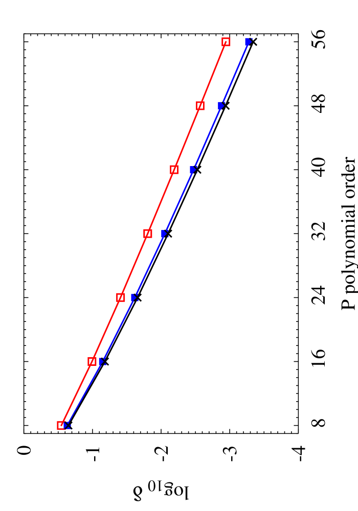
Figure 1: The accuracy level for the P polynomials with different polynomial orders and breakup levels: open squares $n_{b}=1$, filled squares $n_{b}=4,$ crosses $n_{b}=8$ ($am=0.10$).

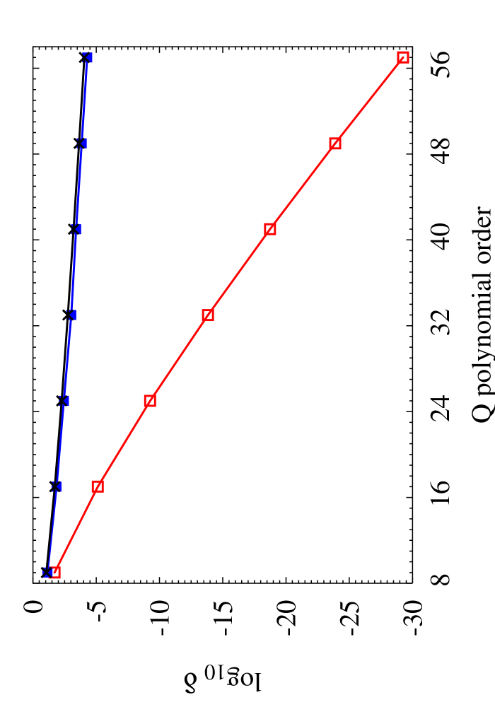
Figure 2: Same as figure 1 but for the Q polynomials.

In order to get a measure of the accuracy of the polynomial approximation we used the distance function $\delta=\sqrt{\delta^{2}}$ defined in Eq. 18 with the weight function set to $\rho\left(x\right)=1$. We have found that it is sufficient to get polynomials with $\delta\sim 10^{-8}$; beyond that the roundoff errors become dominant. In figures 1 and 2 we plot the accuracy of the $\left[P^{\left(n_{b}\right)}_{k}\right]^{n_{b}}$ and $\left[Q^{\left(n_{b}\right)}_{l}\right]^{n_{b}}$ polynomials for $n_{b}=1$, 4 and 8 as the function of the polynomial order for $am=0.1$. The $n_{b}=1$ case is of no practical interest, we show it only to provide a reference. The first thing we notice is that the level of the approximation for the final functions does not increase dramatically as we increase the breakup level. This is startling at first since the resulting polynomial has an order of $n_{b}\times k$, with $k$ the polynomial order. However, if we think that the level of the approximation is determined by the number of the coefficients varied in the minimization procedure this fact is no longer that mysterious. Secondly, we would like to point out that for $n_{b}>1$ the accuracy of the $P_{k}^{\left(n_{b}\right)}$ and $Q_{l}^{\left(n_{b}\right)}$ polynomials with $k\simeq l$ is approximately the same. Thus, there is really no point in using polynomials with $k$ and $l$ vastly different since the level of the accuracy of the final result is going to be dominated by the smaller order polynomial. From figures 1, 2, it is clear that in order to achieve the needed approximation level we have to use polynomials with $k,l\sim 100-200$. The necessary order increases with decreasing quark mass.

Due to the errors introduced by the polynomials the stochastic estimator will not be one even when we do not change the configuration at all ($\Omega=\Omega^{\prime}$) . This is due to the fact that $P\left(x\right)Q\left(x\right)P\left(x\right)$ is not exactly one. This problem can be largely corrected by rewriting the estimator as

$$\xi^{*}[\Omega_{r}^{-1/2n_{b}}(V^{\prime})\Omega_{r}^{1/n_{b}}(V)\Omega_{r}^{-1/2n_{b}}(V^{\prime})-1]\xi\simeq\xi^{*}P_{k}^{(n_{b})}(\Omega^{\prime})[Q_{l}^{(n_{b})}(\Omega)-Q_{l}^{(n_{b})}(\Omega^{\prime})]P_{k}^{(n_{b})}(\Omega^{\prime})\xi.$$ (19)

The right hand side of the expression above has only second order errors. It is a much better approximation of the quantity on the left hand side than the estimator that we get by simply replacing $\Omega_{r}$ with the polynomial approximation. This step is very important since the polynomial approximation would otherwise require much larger order polynomials.

The necessary order for the polynomials $P$ and Q vary with the quark mass but we found that in most cases fairly low orders are sufficient. In simulations with parameters listed in tables 1 and 2 the systematical errors from 128-196 order polynomials were at the same order as numerical round-off errors. However this precision is usually unnecessary. All we need to know for the accept-reject step is whether the stochastic determinant estimate is smaller or greater than a random number; the precise value is not important.

We used a two step approach: we first calculate the stochastic determinant using low order polynomials and we fall back, i.e recalculate the stochastic estimator with higher precision, only if the random number differs from the low order value by less than the estimated error. This method reduces cost if the fall-back rate is small, less or around 10%. To determine the optimum small polynomials we vary their order to minimize the average computational cost.

We estimate the error the low order polynomials might cause from preliminary short runs. A typical short run has a couple of hundreds estimator measurements using the small and the exact (large) polynomials. From this we determine the error of the small polynomials such that the values predicted with small and large polynomials agree within this error at least 99.5% of the time in the production runs.

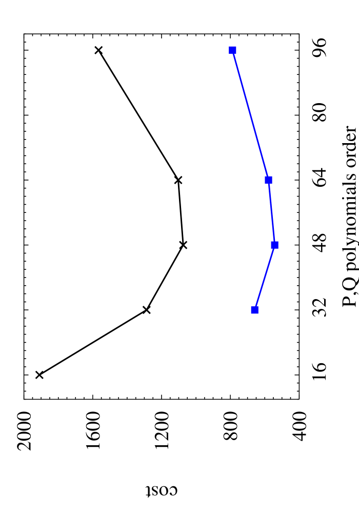
Figure 3: Average computational cost (number of $M^{\dagger}M$ multiplies) for different small polynomials: filled squares $n_{b}=4$, crosses $n_{b}=8$ ($am=0.04$, $k,l\sim 128$ for large polynomials).

We found that the order of the optimum small polynomials is independent of the breakup level, as we can see from figure 3, but the necessary order increases as we decrease the mass. The optimum low order polynomials we determined to be $k=24,$ $l=25$ for quark mass $am=0.1$, $k=32$, $l=33$ for $am=0.06$ and $k=48$, $l=49$ for $am=0.04$. The fall-back rate, i.e. the rate when we had to repeat the stochastic estimator calculation with higher order polynomials varied between 5% and 10%. The outcome of the accept/reject step changed even less frequently, about 10% of the time the fall-back occurred.

The polynomial approximation is a major part of our simulation. Any improvement that reduces the necessary polynomial order or the fall-back rate will immediately reduce the computer time requirements. At present we are investigating several possibilities along this direction.

IV The effectiveness of the partial-global stochastic update

The effectiveness of the PGSM algorithm depends on both the partial-global heat bath update and the stochastic estimator. The autocorrelation time of the simulation is the larger of the autocorrelation times of the heat bath and stochastic steps. If only a small part of the original links are updated, the fermionic matrix ratio $\Omega^{-1}(V^{\prime})\Omega(V)$ is close to unity, the standard deviation and the autocorrelation time of the stochastic estimator is small. On the other hand the heat bath update is ineffective and has to be repeated many times to update the configuration. Inversely, if many links are changed at once, the heat bath update is effective but the standard deviation of the stochastic estimator increases, increasing the autocorrelation time again. We would like to find the optimal update where the simulation is most effective.

We have measured the integrated autocorrelation time of the plaquette as the function of the number of links updated at one heat bath step, $t_{HB}$, both for $n_{f}=4$ and $n_{f}=2$ flavor simulations. The estimates for $\tau_{\rm{auto}}$ in the following are based on runs that were 80-100 times longer than $\tau_{\rm{auto}}$ itself (except at the largest $\tau_{\rm{auto}}$ values where the statistics is smaller). While that does not provide a very good estimate for the autocorrelation, it is sufficient to distinguish the heatbath versus stochastic estimator dominated regions.

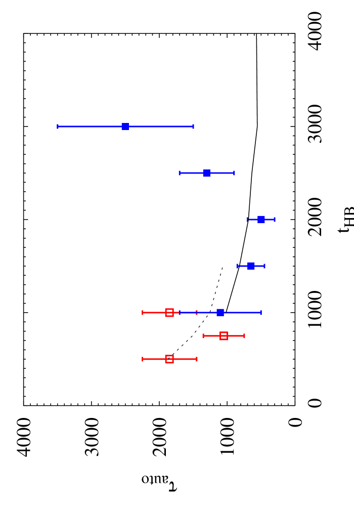
Figure 4: Autocorrelation of the $n_{f}=4$, $am=0.1$ runs. Open squares: $n_{b}=4$ , filled squares: $n_{b}=8$ determinant breakup. The lines correspond to the expected autocorrelation based on the heatbath update alone.

The autocorrelation time of the pure gauge partial-global heat bath update is easy to estimate. If at each step we update $t_{HB}$ links of a lattice of volume V with acceptance rate $r_{a}$, the autocorrelation time $\tau_{pg}$ is related to the autocorrelation time of the whole lattice pure gauge heat bath update $\tau_{HB}$ as

$$\tau_{pg}=\tau_{HB}\frac{4V}{t_{HB}r_{a}}.$$ (20)

In our simulations at $\beta=5.65$ on $8^{3}\times 24$ volumes $\tau_{HB}\sim 10$. The acceptance rate of the PGSM depends not only on $t_{HB}$ but on the determinant breakup parameter $n_{b}$ as well.

The simulation parameters are those listed in tables 1, 2. We considered $n_{b}=4$ and 8 determinant breakup with the $n_{f}=4$, $am=0.1$ runs. The open squares in figure 4 show the autocorrelation time for $n_{b}=4$, the filled squares for $n_{b}=8$.

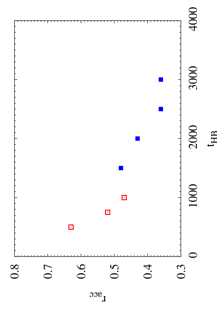
Figure 5: Acceptance rate of the $n_{f}=4$, $am=0.1$ runs. Notation as in figure 4.

The dashed line is $\tau_{pg}$ of Eq. 20 for $n_{b}=4$, the solid line for $n_{b}=8$. For small $t_{HB}$ values both $n_{b}=4$ and 8 follow the $\tau_{pg}$ curve, indicating that the autocorrelation time is dominated by the heatbath step. The $n_{b}=4$ data break off around $t_{HB}=1000$, the $n_{b}=8$ around $t_{HB}=2500$ signaling that the autocorrelation time beyond that is dominated by the stochastic estimator. The acceptance rate, shown in figure 5, varies between 35% and 65% but does not indicate whether the autocorrelation is heatbath or stochastic estimator dominated. For an effective simulation one should choose $t_{HB}=750$ with $n_{b}=4$ or $t_{HB}=2000$ with $n_{b}=8$. Which of these is more effective depends on the implementation of the polynomial approximation in the determinant breakup. In our simulations updating 2000 links with $n_{b}=8$ is the better choice. One should note that at this mass value the $n_{b}=4$ determinant breakup is just barely adequate to guarantee the finiteness of the standard deviation of the stochastic estimator, one more reason to choose $n_{b}=8$ in the simulations.

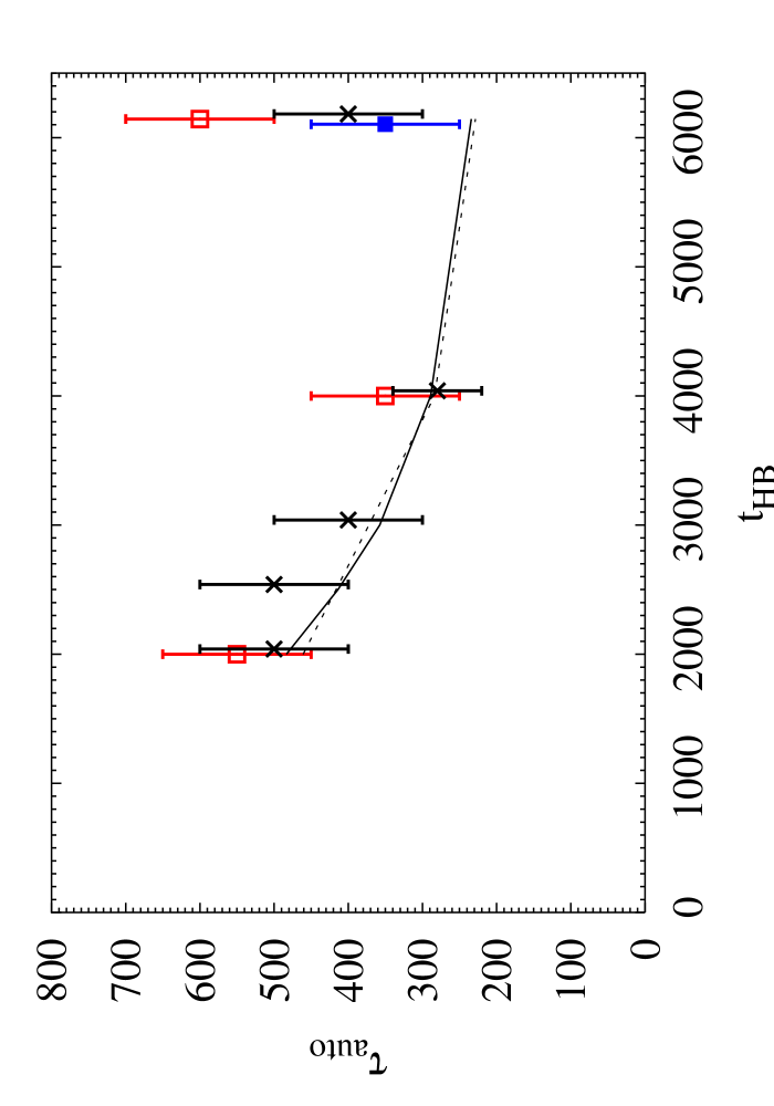
Figure 6: Autocorrelation of the $n_{f}=2$ runs. Open squares: $n_{b}=8$, $am=0.1$, filled squares: $n_{b}=12$, $am=0.1,$ crosses: $n_{b}=12$, $am=0.04$ runs. For clarity the data points are slightly displaced horizontally. The lines corresponds to the expected autocorrelation based on the heatbath update alone. Solid line: $n_{b}=8$, $am=0.1$, dashed line: $n_{b}=12$, $am=0.04$.

The $n_{f}=2$ flavor simulations are considerably more effective. In figure 6 we plot $\tau_{\rm{auto}}$ for the $am=0.1$ mass with $n_{b}=8$ and $n_{b}=12$ and for the $am=0.04$ quark mass with $n_{b}=12$ determinant breakup. Note that the data points with $t_{HB}=6144$ touch the maximum number of links allowed on these $8^{3}\times 24$, close to 10 fm⁴ lattices. With both quark mass values only this last point shows any deviation from the $\tau_{pg}$ heatbath curve. The acceptance rate is shown in figure 7. It is interesting to note that the $am=0.1$ runs with $n_{b}=8$ determinant breakup have very similar acceptance rates to the $am=0.04$, $n_{b}=12$ runs indicating how the determinant breakup should increase with decreasing quark mass. We found similar correspondence in other quantities, like the standard deviation of the stochastic determinant estimate or the average of the action difference $\Delta S$.

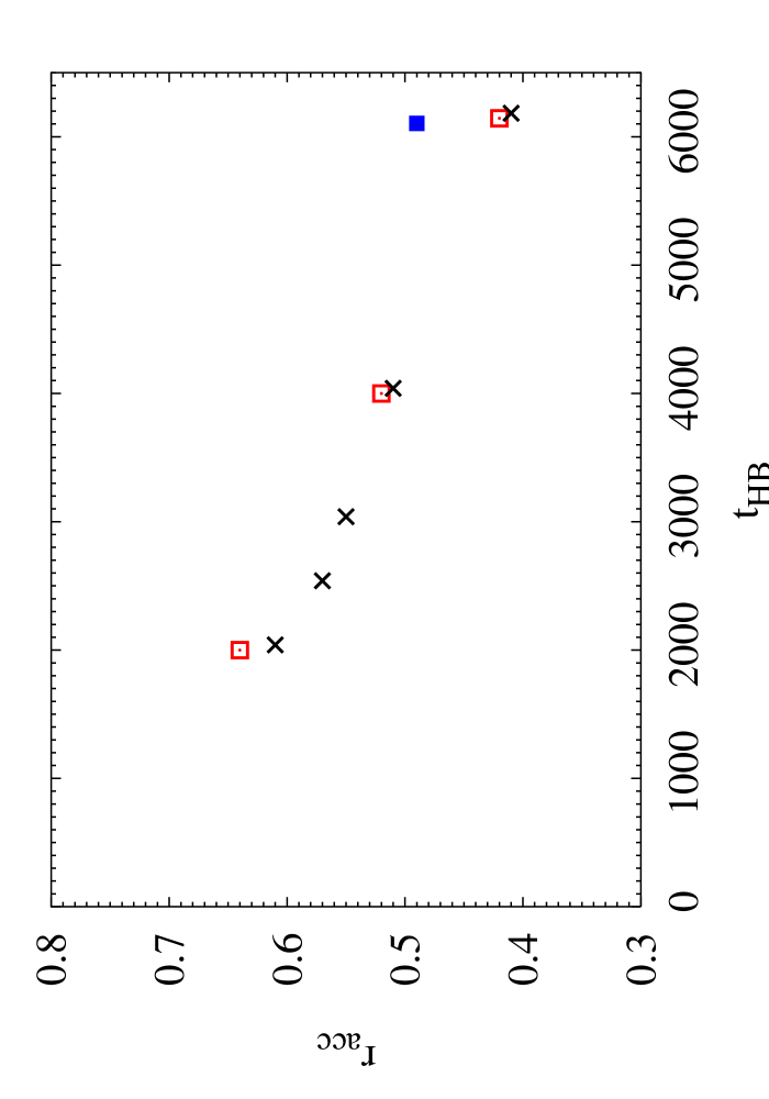
Figure 7: The acceptance rate of the $n_{f}=2$ runs. Notation as in figure 6.

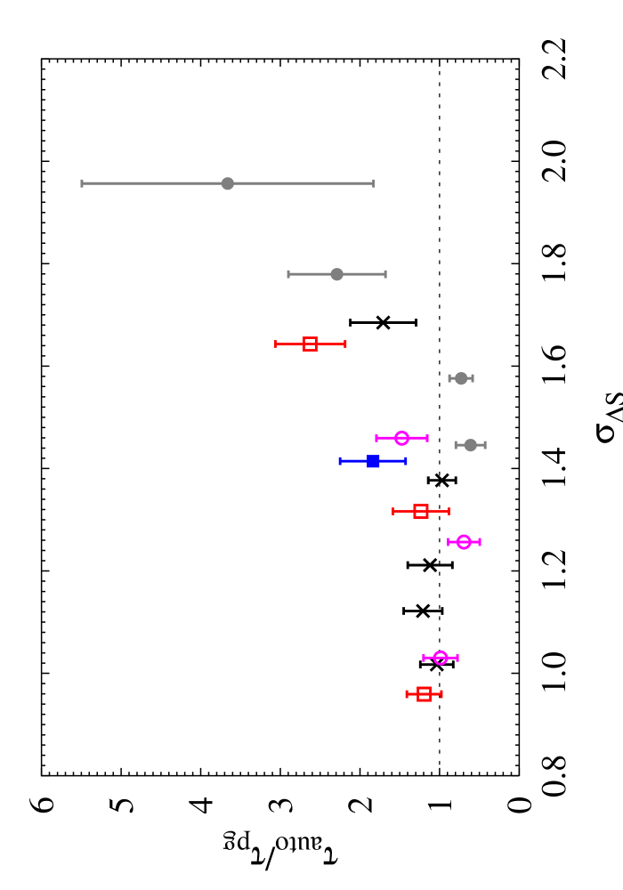
Figure 8: The autocorrelation time in units of $\tau_{pg}$ of Eq. 20 as the function of the standard deviation of the stochastic action, $\Delta S$. Open and filled circles: $n_{f}=4$, $am=0.1$, $n_{b}=4$ and 8 runs. Open and filled squares: $n_{f}=2$, $am=0.1$, $n_{b}=8$ and 12 runs. Crosses: $n_{f}=2$, $am=0.04$, $n_{b}=12$ runs.

Measuring the autocorrelation time requires long simulations. One of our goals in this paper is to find an alternate quantity that is easy to measure but still indicates the crossover from the heatbath to stochastic estimator regions. We have considered the standard deviation of the stochastic estimator and also the standard deviation of $\Delta S$ as defined in Eq. II.4. We decided to use the latter as $\Delta S$ has an almost Gaussian distribution and its standard deviation is easier to estimate. In figure 8 we show both the $n_{f}=4$ and $n_{f}=2$ data for the autocorrelation, measured in units of $\tau_{pg}$, as the function of $\sigma_{\Delta S}=\sqrt{<\Delta S^{2}>-<\Delta S>^{2}}$. As we have already expected from figures 4 and 6, most data points are consistent with $\tau_{\rm{auto}}/\tau_{pg}=1$, i.e. heatbath dominated. We see a gradual increase only at $\sigma_{\Delta S}\geq 1.6$. Based on figures 5,7 and 8 we conclude that the PGSM update is heatbath dominated if the acceptance rate is around 50% or higher and the standard deviation of the action difference $\sigma_{\Delta S}$ is less than about 1.6.

We conclude this section by translating the autocorrelation time measurements to computer time requirements. In figure 9 we plot the computer time measured in fermionic matrix $M^{\dagger}M$ multiplies to create configurations in the $n_{f}=2$ flavor simulations that are separated by $2\tau_{\rm{auto}}$ update steps. These estimates strongly depend on the polynomial approximation but still give a fair indication of the expected computer cost. One should note that in figure 9 we consider the time requirement of the stochastic estimator only. Updating the gauge field and evaluating the HYP smeared links can result in a 10-20% overhead on smaller lattices. In Ref. Hasenfratz and Knechtli (2002) it was found that a HMC thin link staggered fermion update with $n_{f}=4$ flavors at similar physical parameter values to our $am=0.1$ run requires about $1.2\times 10^{6}$ $M^{\dagger}M$ multiplies to create independent configurations . A two flavor run is faster but even than it is evident that on these 10 fm⁴ lattices it is actually faster to create HYP smeared configurations with PGSM than think link ones with a small step-size algorithm.

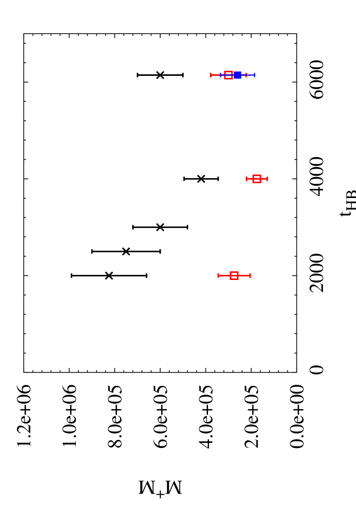
Figure 9: Cost of creating independent configurations, measured in fermionic matrix multiplies. Notation is the same as in figure 6, open squares: $n_{b}=8$, $am=0.1$, filled square: $n_{b}=12$, $am=0.1,$ crosses: $n_{b}=12$, $am=0.04$ runs..

The autocorrelation measurements and computer time estimates presented above were based on runs on 10 fm⁴ lattices. The PGSM algorithm scales with the square of the lattice volume. To repeat the above measurements on 100 fm⁴ lattices would increase the computer time by 100. A factor of 10 increase is due to the increased volume, and the other factor of 10 is coming from the increased autocorrelation time. Simulation cost at smaller lattice spacing but same physical volume increases only linearly with the volume as the number of links that can be effectively touched increases accordingly.

V Conclusion

In this paper we discussed the practical implementation of the partial-global stochastic Metropolis (PGSM) algorithm for HYP link staggered fermions. The PGSM is a two step algorithm where a partial set of the original gauge links are updated with a heatbath or overrelaxed step and this proposed configuration is accepted or rejected according to a stochastic estimate of the fermionic determinant. Even though only a stochastic estimator is used in the Metropolis step, the algorithm satisfies detailed balance.

The effectiveness of the algorithm depends on the matching of the dynamical action and the pure gauge action used in the first step of the algorithm, and on the stochastic estimator used in the Metropolis accept-reject step. The first condition can be met by separating the pure gauge action into a part that depends on the thin gauge links and matches the short and/or long distance properties of the dynamical action, and a part that depends on the smeared links and compensates for the renormalization of the pure gauge coupling due to the dynamical fermions. Only the former is used to propose the new configuration, the latter is included in the accept-reject step. The stochastic estimator can be significantly improved by fermionic matrix reduction and determinant breakup. Our $n_{f}=2$ flavor simulations indicate that with these improvements up to 1 fm⁴ section of the lattice can be updated at one time. The update has to be repeated enough times to refresh the whole lattice, but beyond that the properties of the heatbath update determine the autocorrelation time. Combining the heatbath update with overrelaxation could provide an even more effective algorithm that decorrelates the configurations much faster than the traditional small step size algorithms.