Abstract

An algorithm to simulate full QCD with 3 colours at nonzero chemical potential on the lattice is proposed. The algorithm works for small values of the chemical potential and can be used to extract expectation values of CPT invariant operators.

1 Introduction

Understanding the properties of matter at nonzero density and temperature is an essential ingredient to describe the physics of the early universe and the collapse of very massive stars [1]. Moreover recent heavy ion collision experiments offer a unique laboratory test for the predictions of the theory [2].

Effective models [1, 3] predict a rich structure in the temperature–chemical potential $T$–$\mu$ diagram of QCD with several phases. Numerical simulations on the lattice is an adequate technique to study the corresponding phase transitions. The lattice action of QCD at finite $\mu$ has been given in [4, 5]. By using Wilson fermions within a $SU(N)$ invariant gauge theory, this action is [6]

$$S_{\rm Wilson} \equiv \beta\sum_{P}\left(1-{1\over N}\hbox{Re Tr}\,{P}\right)$$

$$+\sum_{\rm flavours}\sum_{x}a^{3}\Big{[}\left(am+4\lambda\right)\overline{\psi}_{x}\psi_{x}$$

$$\qquad\qquad\qquad-{1\over 2}\sum_{\nu}\Big{(}\left(\lambda-\gamma_{\nu}\right)\overline{\psi}_{x}U_{\nu}(x)\xi_{\nu}(\mu)\psi_{x+\hat{\nu}}$$

$$\qquad\qquad\qquad+\left(\lambda+\gamma_{\nu}\right)\overline{\psi}_{x+\hat{\nu}}U^{\dagger}_{\nu}(x)\xi_{\nu}(\mu)^{-1}\psi_{x}\Big{)}\Big{]}\;,$$

$$\xi_{\nu}(\mu) \equiv 1+\delta_{4\nu}\left(\exp\left(f(a\mu)\right)-1\right)\;,$$ (1)

where the first term is the pure gauge action, $a$ is the lattice spacing, $\beta$ is the inverse bare lattice coupling ($\beta=2N/g_{0}^{2}$), ${P}$ stands for the elementary plaquette, $m$ is the fermion mass, $\lambda$ is the Wilson parameter and $\mu$ is the chemical potential. $f(a\mu)$ is an odd function of the chemical potential that satisfies $f(x)=x+O(x^{3})$. The simplest choice is $f(x)=x$ although others are possible (see for instance [7] where $f(x)=\hbox{arg tanh}x$). Notice that $\xi_{\nu}(-\mu)=\xi_{\nu}(\mu)^{-1}$. Analogous expressions are valid for staggered and naïve fermions.

The expectation value of an operator $O$ is defined by the Feynman path integral

$$\langle O\rangle = {1\over Z}\int{\cal D}U_{\nu}{\cal D}\overline{\psi}_{x}{\cal D}\psi_{x}\;O\,\exp\left(-S_{\rm Wilson}\right)\;,$$

$$Z \equiv \int{\cal D}U_{\nu}{\cal D}\overline{\psi}_{x}{\cal D}\psi_{x}\;\exp\left(-S_{\rm Wilson}\right)\;,$$ (2)

where terms regarding gauge fixing have been skipped as they are inessential for our analysis. After integrating out fermions (we assume that $O$ can be expressed in terms of gluon fields only) we have

$$\langle O\rangle={1\over Z}\int{\cal D}U_{\nu}\;O\,\det D\;\exp\left(-S_{\rm g}\right)\;,$$ (3)

where $S_{\rm g}$ is the pure gauge action and $D$ is the fermion matrix

$$D_{xy}(\mu) = (ma+\lambda)\delta_{x,y}$$

$$-{1\over 2}\negthinspace\negthinspace\negthinspace\negthinspace \negthinspace\negthinspace\negthinspace\negthinspace\sum_{\nu}\left(\delta_{x,y+\hat{\nu}}U^{\dagger}_{\nu}(y)\left(\lambda+\gamma_{\nu}\right)\xi_{\nu}(\mu)^{-1}+\delta_{y,x+\hat{\nu}}U_{\nu}(x)\left(\lambda-\gamma_{\nu}\right)\xi_{\nu}(\mu)\right)\;.$$ (4)

Colour, flavour and spinor indices are placed where required. The theory with $N=3$ colours and fermions in the fundamental representation in general yields a complex value for $\det D$ if $\mu\not=0$. This is a problem because importance sampling in the Monte Carlo integration of Eq.(3) cannot be applied with a complex weight. Several solutions have been proposed that allow to perform the integration in an approximate way or in particular regions of the $T$–$\mu$ diagram: reweighting methods [8], calculation of the canonical partition function from simulations at imaginary chemical potential [9], analytical continuations of Taylor expansions in powers of imaginary chemical potential [10], responses of several observables to a nonzero small chemical potential [11] and fugacity expansions [12]. Here we present another idea that should work for small values of the chemical potential. We will prove that if we restrict our attention to the calculation of expectation values of CPT invariant operators then the correct Boltzmann weight under the path integral is $\exp\left(-S_{\rm g}\right)\hbox{Re}\det D$.

2 The Boltzmann weight

The Boltzmann weight in Eq.(3), $\exp\left(-S_{\rm g}\right)\det D$, is a complex number. However the expectation value of any observable represented by the operator $O$ in Eq.(3) must be a real quantity. Imposing that $\langle O\rangle$ be real for any observable $O$ is a strong constraint on the integration measure. Clearly all possible configurations can be gathered in sets such that the contribution to the imaginary part of $\langle O\rangle$ from all configurations in one single set cancels out. We shall assume that all sets are formed by only two configurations and that these two are related by some transformation S. Firstly we want to find this transformation. Let ${\cal C}$ denote a thermalized arbitrary configuration on the lattice and ${\cal C^{\sf S}}$ the corresponding transformed configuration by the action of S. We require that (i) the value of the operator $O$ calculated on ${\cal C}$ and ${\cal C^{\sf S}}$ be the same; (ii) the weight under the path integral for ${\cal C^{\sf S}}$ be the complex conjugate of the weight for ${\cal C}$ and (iii) ${\cal C}$ and ${\cal C^{\sf S}}$ have the same Haar measure,

$$O[{\cal C}] \rightarrow O[{\cal C^{\sf S}}]=O[{\cal C}]\;,$$

$$\det D[{\cal C}]\hbox{e}^{-S_{\rm g}[{\cal C}]} \rightarrow \det D[{\cal C^{\sf S}}]\hbox{e}^{-S_{\rm g}[{\cal C^{\sf S}}]}=\left(\det D[{\cal C}]\right)^{*}\hbox{e}^{-S_{\rm g}[{\cal C}]}\;,$$

$${\cal D}U_{\nu}[{\cal C}] \rightarrow {\cal D}U_{\nu}[{\cal C^{\sf S}}]={\cal D}U_{\nu}[{\cal C}]\;,$$ (5)

where we have explicitely written the dependence on the configuration. We will write this dependence wherever necessary. These conditions are sufficient to guarantee that $\langle O\rangle$ is real.

A simple way to enforce the last constraint in (5) is by imposing that S is a discrete transformation. ${\cal D}U_{\nu}$ means $\Pi_{x}\Pi_{\nu}\hbox{d}U_{\nu}(x)$ where each single factor $\hbox{d}U_{\nu}(x)$ is the Haar measure over the gauge group. By a discrete transformation we mean that S does not transform each single Haar measure. In fact this would entail a jacobian and the search of the transformed configuration would become more difficult.

The matrix $D_{xy}(\mu)$ has the property $\left(\det D(\mu)\right)^{*}=\det D(-\mu)$. This stems from the relation $D(\mu)^{\dagger}=\gamma_{5}D(-\mu)\gamma_{5}$. Notice that this implies Re det$D$ (Im det$D$) is an even (odd) function of $\mu$. Moreover it is physically clear that applying a charge conjugation operator C changes the sign of $\mu$. Then we expect that the condition $\det D[{\cal C^{\sf S}}]=\left(\det D[{\cal C}]\right)^{*}$ can be verified if S contains the transformation C. However the above condition is only part of the requirements in (5). In particular we see from the second condition in (5) that the implementation of C must be such that the pure gluon action $S_{\rm g}$ remains unaltered.

In order to leave $S_{\rm g}$ invariant, the correct transformation should involve some space–time rearrangement besides charge conjugation. A reasonable guess is the CPT transformation that we define in the following way: if our lattice was $d$ dimensional and the lateral sizes were finite and equal to $L_{1}$, $L_{2}$, …, $L_{d}$ (in units of lattice spacing) then the CPT transformation would act in the following way

$$U_{\nu}(x)^{{\sf CPT}}=U_{\nu}^{\dagger}( \negthinspace\negthinspace\negthinspace\negthinspace\negthinspace\negthinspace\negthinspace\negthinspace\negthinspace\hbox{mod}(L_{1}-x_{1}+1,L_{1})+1,$$ (6)

$$\negthinspace\negthinspace\negthinspace\negthinspace\negthinspace\negthinspace\negthinspace\negthinspace\negthinspace\hbox{mod}(L_{2}-x_{2}+1,L_{2})+1,$$

$$\negthinspace\negthinspace\negthinspace\negthinspace\negthinspace\negthinspace\negthinspace\negthinspace\negthinspace\cdots,$$

$$\negthinspace\negthinspace\negthinspace\negthinspace\negthinspace\negthinspace\negthinspace\negthinspace\negthinspace\hbox{mod}(L_{\nu}-x_{\nu},L_{\nu})+1,$$

$$\negthinspace\negthinspace\negthinspace\negthinspace\negthinspace\negthinspace\negthinspace\negthinspace\negthinspace\cdots,$$

$$\negthinspace\negthinspace\negthinspace\negthinspace\negthinspace\negthinspace\negthinspace\negthinspace\negthinspace\hbox{mod}(L_{d}-x_{d}+1,L_{d})+1)\;,$$

where mod($x,L$) gives the remainder on integer division of $x$ by $L$. This is the finite volume version of $U_{\nu}(x)^{\sf CPT}=U^{\dagger}_{\nu}(-x)$. This transformation fulfils all conditions in Eq.(5) as a straightforward computation shows.

As an example let us check that $S_{\rm g}$ is invariant under CPT. It is enough to show that under the action of CPT every plaquette of the original configuration ${\cal C}$ maps onto one and only one plaquette of ${\cal C}$. Let us denote ${P}(x;\nu,\rho)$ the plaquette starting at the site $x$ and going around through direction $\nu$ and then $\rho$. This is ${P}(x;\nu,\rho)\equiv U_{\nu}(x)U_{\rho}(x+\hat{\nu})U^{\dagger}_{\nu}(x+\hat{\rho})U^{\dagger}_{\rho}(x)$. Applying transformation (6) on each factor we obtain

$${P}(x;\nu,\rho)\rightarrow U^{\dagger}_{\nu} \negthinspace\negthinspace\negthinspace\negthinspace\negthinspace\negthinspace\negthinspace\negthinspace\negthinspace(\hbox{mod}(L_{1}-x_{1}+1,L_{1})+1,\cdots$$

$$\negthinspace\negthinspace\negthinspace\negthinspace\negthinspace\negthinspace\negthinspace\negthinspace\negthinspace\hbox{mod}(L_{\nu}-x_{\nu},L_{\nu})+1,\cdots$$

$$\negthinspace\negthinspace\negthinspace\negthinspace\negthinspace\negthinspace\negthinspace\negthinspace\negthinspace\hbox{mod}(L_{\rho}-x_{\rho}+1,L_{\rho})+1,\cdots)\times$$

$$U^{\dagger}_{\rho} \negthinspace\negthinspace\negthinspace\negthinspace\negthinspace\negthinspace\negthinspace\negthinspace\negthinspace(\hbox{mod}(L_{1}-x_{1}+1,L_{1})+1,\cdots$$

$$\negthinspace\negthinspace\negthinspace\negthinspace\negthinspace\negthinspace\negthinspace\negthinspace\negthinspace\hbox{mod}(L_{\nu}-x_{\nu},L_{\nu})+1,\cdots$$

$$\negthinspace\negthinspace\negthinspace\negthinspace\negthinspace\negthinspace\negthinspace\negthinspace\negthinspace\hbox{mod}(L_{\rho}-x_{\rho},L_{\rho})+1,\cdots)\times$$

$$U_{\nu} \negthinspace\negthinspace\negthinspace\negthinspace\negthinspace\negthinspace\negthinspace\negthinspace\negthinspace(\hbox{mod}(L_{1}-x_{1}+1,L_{1})+1,\cdots$$

$$\negthinspace\negthinspace\negthinspace\negthinspace\negthinspace\negthinspace\negthinspace\negthinspace\negthinspace\hbox{mod}(L_{\nu}-x_{\nu},L_{\nu})+1,\cdots$$

$$\negthinspace\negthinspace\negthinspace\negthinspace\negthinspace\negthinspace\negthinspace\negthinspace\negthinspace\hbox{mod}(L_{\rho}-x_{\rho},L_{\rho})+1,\cdots)\times$$

$$U_{\rho} \negthinspace\negthinspace\negthinspace\negthinspace\negthinspace\negthinspace\negthinspace\negthinspace\negthinspace(\hbox{mod}(L_{1}-x_{1}+1,L_{1})+1,\cdots$$

$$\negthinspace\negthinspace\negthinspace\negthinspace\negthinspace\negthinspace\negthinspace\negthinspace\negthinspace\hbox{mod}(L_{\nu}-x_{\nu}+1,L_{\nu})+1,\cdots$$

$$\negthinspace\negthinspace\negthinspace\negthinspace\negthinspace\negthinspace\negthinspace\negthinspace\negthinspace\hbox{mod}(L_{\rho}-x_{\rho},L_{\rho})+1,\cdots)\;,$$

which, by the cyclic property of the trace, is equivalent to the plaquette

$${P}(\hbox{mod}(L_{1}-x_{1}+1,L_{1})+1,\cdots,\hbox{mod}(L_{\nu}-x_{\nu},L_{\nu})+1,\cdots,$$

$$\quad\,\hbox{mod}(L_{\rho}-x_{\rho},L_{\rho})+1,\cdots,\hbox{mod}(L_{d}-x_{d}+1,L_{d})+1;\nu,\rho)$$ (8)

in the original configuration ${\cal C}$. This is clearly a one–to–one mapping from plaquettes to plaquettes in ${\cal C}$. This completes the proof.

Then a configuration ${\cal C}$ with weight $\det D\exp(-S_{\rm g})$ transforms under CPT into another configuration ${\cal C}^{{\sf CPT}}$ with weight $\left(\det D\right)^{*}\exp(-S_{\rm g})$ and the same Haar measure. This means that both configurations have the same odds to be selected by an updating algorithm. If moreover we restrict our interest only to CPT invariant observables $O$ then we can say that the numerical value $O[{\cal C}]$ appears with a probability proportional to $\exp(-S_{\rm g}[{\cal C}])\left(\det D[{\cal C}]+\left(\det D[{\cal C}]\right)^{*}\right)$. Barring a factor 2 and dispensing with the CPT transformed configuration one can just count ${\cal C}$ with the weight $\exp(-S_{\rm g})\hbox{Re}\det D$. This is the main result of our paper.

When we say CPT invariant operators we mean that the operator $O$ is CPT invariant configuration by configuration. Most of the operators are CPT invariant after averaging over configurations (i.e. the corresponding observable is CPT invariant), but our constraint is stronger than this.

Focusing our attention only on CPT invariant operators still allows to study several interesting problems. Indeed the average plaquette, chiral condensate, Polyakov loop, etc. can be calculated by evaluating expectation values of CPT invariant operators. On the other hand space–time valued operators $O(x)$ are in general not permitted because our method requires that the equality $O(x)=O(-x)^{\dagger}$ holds configuration by configuration which in general is not true. In particular all correlation functions are not admissible.

Are there other discrete transformations such that the imaginary part of the determinant is eliminated within groups of two configurations? We have performed the following test. We discretized a 2–dimensional gauge theory on a $2^{2}$ lattice and loaded it with an arbitrary configuration (an arbitrary $SU(3)$ matrix on each of the 8 links). We calculated $\det D$ obtaining a complex number. Then we rearranged the 8 $SU(3)$ matrices in all possible ways (8!=40320) and for each permutation we placed them again on the 8 links and recalculated the determinant. Only the transformation described in (6) yielded the result that satisfies conditions (5) (permutations of the 8 links that can be viewed as spatial or temporal translations led to the same result but they are clearly uninteresting). We conclude that there are no other simple discrete transformations providing the complex conjugate of the original configuration weight.

3 A note on Monte Carlo simulation

For the importance sampling to work it is necessary that the weight be positive (it must behave as a probability). However Re $\det D$ can take negative values and this fact limits the applicability of the method. By continuity we expect that Re $\det D$ is positive in the majority of configurations when $\mu$ is small enough. This suspicion is confirmed by numerical simulation. In [13] results from a simulation with 4 flavours of staggered fermions are presented. A $4^{4}$ lattice is used at $\beta=4.8$ and $am=0.025$. In Fig. 1 we show the fraction of configurations with a positive (negative) weight $N_{+}/N$ ($N_{-}/N$) as a function of $a\mu$ ($N\equiv N_{+}+N_{-}$ is the total number of configurations). It indicates that our method can be used at moderate values of $\mu$. This may include the region in the phase diagram $T$–$\mu$ where present and future heavy ion experiments (RHIC, LHC) are going to be run (large $T$ and small $\mu$).

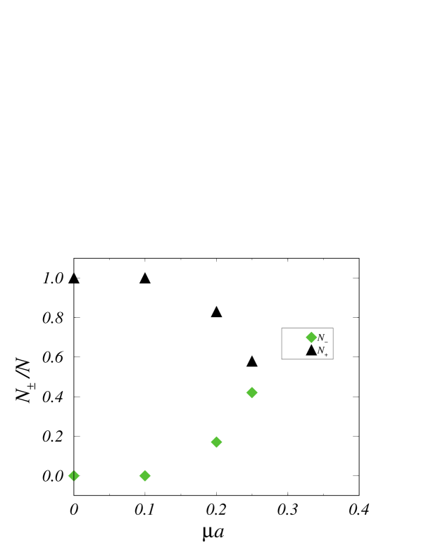
Figure 1: Fraction of positive and negative weighted configurations as a function of the chemical potential. Data taken from [13].

Monte Carlo simulations with the weight Re $\det D$ would be greatly facilitated if we were able to find a new matrix $\Delta$ such that Re $\det D=\det\Delta$ because then fast and well–known simulation methods for fermions [14] could be used. We have not found a general and efficient algorithm to construct the matrix $\Delta$ starting from $D$. Consequently we have to resort to algorithms which explicitely calculate the determinant of $D$.

We shall not insist in these aspects of the problem as they will be analysed in a future publication containing several numerical studies [15].

4 Conclusions

We have proved that the correct Boltzmann weight for updating full QCD in lattice simulations at finite chemical potential is

$$\exp\left(-S_{\rm g}\right)\hbox{Re }\det D$$ (9)

where $S_{\rm g}$ is the pure gluon action and $D$ is the fermion matrix. We have shown that this is true when we calculate expectation values of operators that are CPT invariant. For other operators our proof does not work. Possibly in this case the assumption that the imaginary part of the Boltzmann weight is eliminated by combining couples of configurations should be relaxed. Nonetheless the class of CPT invariant operators include many observables usually studied in the context of finite density systems.

Our algorithm has two problems which deserves further improvement: on one hand the weight (9) is not positive in general. We have shown that it is mostly positive for moderate values of the chemical potential. On the other hand the present method requires the explicit calculation of the determinant of the fermion matrix $D$ which is very time consuming. In a future publication [15] we will give numerical results obtained by using Eq.(9).

5 Acknowledgements

It is a pleasure to thank G. Marchesini for useful discussions.

References

- [1] See for instance K. Rajagopal, F. Wilczek, hep–ph/0011333; G. Nardulli, hep–ph/0206065.
- [2] H. Satz, Nucl. Phys. B (Proc. Suppl.) 94 (2001) 204; R. V. Gavai, hep–ph/0010048.
- [3] B. Barrois, Nucl. Phys. B129 (1977) 390; D. Bailin, A. Love, Phys. Rep. 107 (1984) 325; R. Casalbuoni, R. Gatto, G. Nardulli, Phys. Lett. B498 (2001) 179.
- [4] P. Hasenfratz, F. Karsch, Phys. Lett. B125 (1983) 308.
- [5] J. Kogut, H. Matsuoka, M. Stone, H. W. Wyld, S. Shenker, J. Shigemitsu, D. K. Sinclair, Nucl. Phys. B225 [FS9] (1983) 93.
- [6] K. G. Wilson, Phys. Rev. D10 (1974) 2445; in “New Phenomena in Subnuclear Physics”, ed. A. Zichichi (Plenum Press, New York) (1975) pg. 69.
- [7] N. Bilic, R. V. Gavai, Z. Phys. C23 (1984) 77.
- [8] Z. Fodor, S. D. Katz, hep–lat/0204029.
- [9] M. Alford, A. Kapustin, F. Wilczek, Phys. Rev. D59 (1999) 054502.
- [10] Ph. de Forcrand, O. Philipsen, hep–lat/0205016; M. D’Elia, M.–P. Lombardo, hep–lat/0205022.
- [11] S. Choe, Ph. de Forcrand, M. García–Pérez, S. Hioki, Y. Liu, H. Matsufuru, O. Miyamura, I.-O. Stamatescu, T. Takaishi, T. Umeda, Nucl. Phys. B (Proc. Suppl.) 106 (2002) 462; C. R. Allton, S. Ejiri, S. J. Hands, O. Kaczmarek, F. Karsch, E. Laermann, Ch. Schmidt, L. Scorzato, hep–lat/0204010.
- [12] I. M. Barbour, C. T. H. Davies, Z. Sabeur, Phys. Lett. B215 (1988) 567.
- [13] D. Toussaint, Nucl. Phys. B (Proc. Suppl.) 17 (1990) 248.
- [14] S. Gottlieb, W. Liu, D. Toussaint, R. L. Renken, R. L. Sugar, Phys. Rev. D35 (1987) 2531.
- [15] B. Allés, E. M. Moroni, in preparation.