Supersymmetry on a Spatial Lattice

Abstract:

We construct a variety of supersymmetric gauge theories on a spatial lattice, including $N=4$ supersymmetric Yang-Mills theory in 3+1 dimensions. Exact lattice supersymmetry greatly reduces or eliminates the need for fine tuning to arrive at the desired continuum limit in these examples.

1 Searching for accidental supersymmetry

There are numerous fascinating features in strongly coupled supersymmetry, supergravity and string theory that would benefit from numerical investigation. Furthermore, it is desirable to know whether a well defined nonperturbative description of these theories exists. For these reasons much effort has been devoted to the formulation of lattice versions of supersymmetric field theories [1, 2, 3, 4, 5, 6, 7, 8, 9, 10, 11, 12, 13, 14, 15, 16, 17, 18]. To date, this work has led to limited practical success, confined primarily to some $1+1$ dimensional theories, or $N=1$ supersymmetric Yang-Mills (SYM) theory in $3+1$ dimensions.

The origin of the problem is that supersymmetry is part of the super-Poincaré group, which is explicitly broken by the lattice. Ordinary Poincaré invariance is also broken by the lattice, but due to the crystal symmetry of the lattice, relevant operators which could spoil the emergence of Poincaré symmetry in the continuum limit are forbidden. In a supersymmetric theory, however, the lattice point group is never sufficient to forbid relevant supersymmetry violating operators.

One would like to implement exact symmetries on the lattice that ensure that supersymmetry emerges as an “accidental” continuum symmetry of the theory. In four dimensions, accidental supersymmetry can be achieved for $N=1$ supersymmetric Yang-Mills (SYM) theory, a theory without spin zero bosons. (See ref. [19] for discussion and references.) This is because for a generic $SU(k)$ gauge theory with an adjoint Weyl fermion, the only relevant operator which violates $N=1$ supersymmetry is a fermion mass term, which can be forbidden by a discrete chiral $Z_{2k}$ symmetry [20]. Thus by using Wilson fermions in the adjoint representation and tuning the fermion mass, one may obtain $N=1$ SYM in the continuum limit [7, 15]. Alternatively, one can implement chiral fermions on the lattice; this approach has been explored in [21, 6, 8, 9, 10, 12, 13, 14] using domain wall [22, 23] or overlap fermions [21, 24] to implement the $Z_{2k}$ chiral symmetry.

In supersymmetric theories with scalar fields, however, there tend to be a plethora of relevant operators which violate supersymmetry. There are no linearly realized symmetries that can forbid some of these operators, such as scalar mass terms, other than supersymmetry itself. Unfortunately, there is no discrete version of supersymmetry analogous to the lattice subgroup of Poincaré symmetry which can be implemented to forbid scalar masses and other unwanted relevant operators, since supersymmetry generators are fermionic and there are no macroscopic supersymmetry transformations. This suggests that a realization of supersymmetry in the continuum would greatly benefit by having some subset of the target theory’s supersymmetry algebra realized exactly on the lattice. This has been the recent approach of refs. [17, 16].

In this paper we discuss a method for implementing supersymmetry on a spatial lattice with continuous Minkowski time. In particular, we show that SYM theories with extended supersymmetry in various dimensions may be constructed on a spatial lattice in a manner that either eliminates or significantly reduces fine tuning problems associated with obtaining the desired target theory. Our method is to start with a “mother theory”, being a quantum mechanical system with extended supersymmetry, a large $N$ gauge symmetry, and a global $R$-symmetry group $G_{R}$ (defined to be the global symmetry group of the theory which does not commute with the supercharges). The spatial lattice is constructed by “orbifolding” by $Z_{N}$ gauge and $R$ symmetries, partially breaking the extended supersymmetry and producing $N$-site lattice dimensions. Subsequently taking the continuum limit of this “daughter theory” near a particular point in the classical moduli space of vacua can result in a higher dimensional quantum field theory with the original extended supersymmetry restored, along with Poincaré invariance. The advantage of this technique is that the resultant lattice can retain some exact supersymmetries, which facilitates recovery of the remaining supersymmetries in the continuum limit, protecting the theory from undesirable radiative corrections.

While the present work is confined to examples of spatial lattices with Minkowski time, there are no obstructions to extending these techniques to Euclidean spacetime lattices, the subject of ref. [25] and subsequent papers in preparation.

The paradigm and motivation for this approach toward lattice supersymmetry is found in the deconstruction of SYM theory in 4+1 dimensions, by Arkani-Hamed, Cohen and Georgi [26, 27] and the deconstruction of certain 5+1 dimensional theories in ref. [28]. Our discussion of lattices derived from the mother theory with sixteen supercharges has some overlap with ref. [29], and some related results were derived from string theory by Arkani-Hamed, Cohen, Karch and Motl (unpublished).

In the next section we discuss how one can start with a “mother” theory with a large symmetry group, and then mod out discrete symmetries (“orbifolding”) to create daughter theories with a lattice structure. In the subsequent section we consider SYM theories with four, eight, and sixteen supercharges in 0+1 dimensions, and the types of lattices that can be obtained from them via orbifolding. We then examine in some detail the simplest of these lattices, and discuss how to obtain from it a continuum supersymmetric quantum field theory—in this case, (2,2) SYM in 1+1 dimensions. The more complicated, higher dimensional theories are subsequently treated, although in less detail. A summary of supersymmetric notation relevant for our analysis is provided a summary in an Appendix, in order to make this paper more readable.

2 Orbifolding

We begin by describing how one can create a supersymmetric lattice action by performing an orbifold projection of a supersymmetric quantum mechanics theory. This seemingly unnecessarily complicated approach to constructing a lattice action is justified by the fascinating and useful properties of the supersymmetric lattices that result from this procedure.

We start with a mother theory in $0+1$ dimensions possessing extended supersymmetry, a gauge group $U(kN^{d})$, and a global $R$ symmetry $G_{R}$. By definition, an $R$-symmetry $G_{R}$ is a global symmetry under which the supercharges transform nontrivially. We will identify the maximal Abelian subgroup of $G_{R}$ to be $H_{R}=U(1)^{p}$, where $p$ is the rank of $G_{R}$. The variables of the daughter theory are then constructed by first identifying a particular $(Z_{N})^{d}$ subgroup of $H_{R}\times U(kN^{d})$, and then projecting out all fields in the mother theory which transform nontrivially under this $(Z_{N})^{d}$ symmetry. The action of the theory is simply determined by replacing all of the fields in the action of the mother theory by their projections. The resultant action can be thought of as a lattice action, where the lattice is $d$-dimensional with $N^{d}$ sites, possessing an independent $U(k)$ gauge symmetry at each site. This technique has been extensively discussed in the literature in other contexts (see, for example [30, 31, 32, 33, 34]). The continuum limit of such a lattice will describe a $d+1$ dimensional quantum $U(k)$ gauge theory. A special feature of the daughter theory lattice is that in the classical continuum limit, all of the supersymmetries of the mother theory are recovered. Furthermore, $2^{-d}$ of the mother theory’s supersymmetries are preserved by the orbifold projection, so that for many of the lattices we construct, there are no relevant operators allowed which would allow quantum effects to spoil the classical continuum limit.

To be explicit, consider an adjoint field $\Phi$ in the mother theory, which is a $kN^{d}\times kN^{d}$ matrix, transforming as $\Phi\to U\Phi U^{\dagger}$ under the $U(kN^{d})$ gauge symmetry. The field $\Phi$ also transforms as some representation ${\cal R}$ under the global symmetry $G_{R}$; it will carry $H_{R}=U(1)^{p}$ charges $(q_{1},\ldots,q_{p})$ whose values will depend on the representation ${\cal R}$. From these $q_{i}$ charges we form $d<p$ linear combinations $\{r_{1},\ldots,r_{d}\}\equiv{\bf r}$, where all $r_{a}$ charges in the theory take on only integer values (we will discuss below how we choose these particular combinations of the $q$ charges). Again, the ${\bf r}$ charges for a given field $\Phi$ which will depend upon its particular $G_{R}$ representation ${\cal R}$. A $Z_{N}^{d}$ symmetry is then identified, whose action on $\Phi$ is

$$\Phi\to e^{-2\pi ir_{a}/N}\gamma_{a}^{-1}\Phi\gamma_{a}\ ,\quad a=1,\ldots,d.$$ (1)

Here the matrix $\gamma_{a}\in U(kN^{d})$ is given by

$$\gamma_{a}=\underbrace{1_{N}\otimes\ldots}_{a-1}\otimes\Omega\otimes\underbrace{1_{N}\otimes\ldots}_{d-a}\otimes 1_{k}\ ,\qquad\Omega=\rm{diag}(\omega^{1},\omega^{2},\ldots,\omega^{N})\ ,$$ (2)

where $1_{N}$ and $1_{k}$ are the $N\times N$ and $k\times k$ unit matrices respectively, with $\omega=e^{2\pi i/N}$. The orbifold projection then discards all field components which transform nontrivially under this $Z_{N}^{d}$, keeping only those which satisfy the $d$ matrix-valued constraints

$$\Phi=e^{-2\pi ir_{a}/N}\gamma_{a}^{-1}\Phi\gamma_{a}\ ,\quad a=1,\ldots,d.$$ (3)

It is convenient to consider $\Phi$ as being composed of $k\times k$ blocks $\phi_{{\bf mn}}$, where ${\bf m}$ and ${\bf n}$ are $d$-component vectors whose integer components each run from $1$ to $N$. The orbifold projection results in forcing all of these $\phi_{{\bf mn}}$ blocks to vanish except those for which

$${\bf n}={\bf m}+{\bf r}\ .$$ (4)

The surviving $\phi_{\bf mn}$ blocks satisfying the condition Eq. (3) are unconstrained, and will be interpreted as lattice variables. Thus in the $a^{th}$ subspace, a field $\Phi$ for which $r_{a}=0$ will have only diagonal blocks survive, while if $r_{a}=\pm 1$, only the super- or sub-diagonal blocks survive.

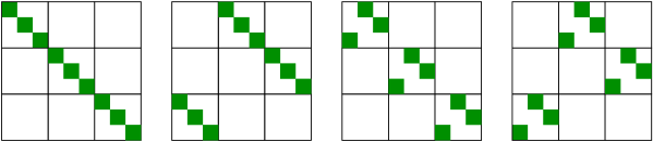
Figure 1: An example of the orbifold procedure in Eq. (3) for a $U(9k)$ gauge group with global symmetry $G_{R}=U(1)\times U(1)$, modded out by $Z_{3}\times Z_{3}$. The dark squares are the $k\times k$ blocks which survive the orbifold projection within a $U(9k)$ adjoint field with $G_{R}$ charges ${\bf r}$. The examples shown (from left to right in the figure) correspond to ${\bf r}=(0,0)$, $(1,0)$, $(0,1)$ and $(1,1)$. The projected fields may be interpreted respectively as fields living on sites, horizontal links, vertical links, and diagonal links on a $3\times 3$ periodic lattice.

When the projected fields satisfying Eq. (3) are substituted into the action of the mother theory, then it becomes a theory of the $N^{d}$ surviving blocks $\phi_{{\bf mn}}$ from each field $\Phi$ of the mother theory. This action is called the daughter theory. The daughter theory (often called a “moose” or a “quiver” in the literature) has a lattice interpretation. The lattice is $d$-dimensional with $N$ sites in each direction, with each surviving $k\times k$ matrix variable $\phi_{\bf mn}$ residing on the link between sites ${\bf m}$ and ${\bf n}$ (or at the site ${\bf m}$ if ${\bf m}={\bf n}$). As the mother theory will possess of a number of different $\Phi$ fields, each with a different ${\bf r}$ charge, the daughter theory will consist of different site and link variables. For $d=2$, for example, fields for which ${\bf r}=\{0,0\}$ will live on lattice sites, while those for which ${\bf r}=\{1,0\}$, $\{0,1\}$ or $\{1,1\}$ will live on horizontal, vertical, or diagonal links respectively . See Fig. 1 for an example.

The orbifold projection breaks the symmetries of the mother theory. For example, general $G_{R}$ transformations which rotate $\Phi$ fields of the mother theory with different ${\bf r}$ charges into each other are broken. The $U(kN^{d})$ gauge symmetry is also broken by the orbifold condition Eq. (3), down to a $U(k)^{N^{d}}$ symmetry. If one considers a general $U(kN^{d})$ matrix as being composed of $N^{2d}$ $k\times k$ blocks $u_{\bf mn}$, then only those transformations consisting solely of diagonal blocks ($u_{\bf mn}=u_{\bf m}\delta_{\bf mn}$) commute with the orbifold condition Eq. (3), where each diagonal block $u_{\bf m}$ is an unconstrained time dependent $U(k)$ matrix associated with the site ${\bf m}$. Under this unbroken $U(k)^{N^{d}}$ symmetry, the lattice variables transform as $\phi_{\bf mn}\to u_{\bf m}\phi_{\bf mn}u^{\dagger}_{\bf n}$, so that a site variable $\phi_{\bf mm}$ transforms as a $U(k)_{\bf m}$ adjoint, while a link variable $\phi_{\bf mn}$ transforms as a bifundamental $(\raisebox{-0.5pt}{\hbox{\rule{0.4pt}{6.5pt}\hskip-0.4pt\rule{6.5pt}{0.4pt}\hskip-6.5pt\rule[6.5pt]{6.5pt}{0.4pt}}\rule[6.5pt]{0.4pt}{0.4pt}\hskip-0.4pt\rule{0.4pt}{6.5pt}},\kern 0.8pt\overline{\kern-0.8pt\raisebox{-0.5pt}{\hbox{\rule{0.4pt}{6.5pt}\hskip-0.4pt\rule{6.5pt}{0.4pt}\hskip-6.5pt\rule[6.5pt]{6.5pt}{0.4pt}}\rule[6.5pt]{0.4pt}{0.4pt}\hskip-0.4pt\rule{0.4pt}{6.5pt}}\kern-0.8pt}\kern 0.8pt)$ under $U(k)_{\bf m}\times U(k)_{\bf n}$. This exact $U(k)^{N^{d}}$ gauge symmetry of lattice (where the gauge transformations depend only on time) becomes a $U(k)$ gauge symmetry in the $d+1$ dimensional field theory that results in the continuum limit, and for each $U(kN^{d})$ adjoint field $\Phi$ of the mother theory, there will result a $U(k)$ adjoint field in the continuum. This method of generating a lattice has created the $d$ spatial dimensions out of the enormous gauge symmetry of the mother theory.

The daughter theory possesses a number of discrete symmetries as well. In general, certain discrete $G_{R}$ transformations which exchange the $H_{R}$ charges $q_{i}$ of the $\Phi$ fields in the mother theory combine with discrete $U(kN^{d})$ symmetries to form the point group of the resulting lattice (see [25] for an explicit example). Another important discrete symmetry of the lattice is a $Z_{N}^{d}$ symmetry which can be interpreted as the group of finite lattice translations. The generators are given by a set of matrices analogous to the $\gamma_{a}$ in Eq. (2), but with the “clock” matrix $\Omega$ replaced by an $N\times N$ “shift” matrix

$$T=\begin{pmatrix}0\ \ &\ \ 1\ \ &&\\ &\,\,\kern-1.5pt\raisebox{4.39166pt}{$\cdot$}\kern 1.5pt\raisebox{0.0pt}{${\mathbf{\cdot}}$}\kern 1.5pt\raisebox{-4.39166pt}{$\cdot$}&\,\,\kern-1.5pt\raisebox{4.39166pt}{$\cdot$}\kern 1.5pt\raisebox{0.0pt}{${\mathbf{\cdot}}$}\kern 1.5pt\raisebox{-4.39166pt}{$\cdot$}&\\ &&\ \ 0\ \ &\ \ 1\ \\ 1\ \ &&&\ \ 0\ \\ \end{pmatrix}\ .$$ (5)

It is straightforward to see that these translation symmetries commute with the orbifold condition Eq. (3). As a consequence of this symmetry, one sees that our orbifold projection results in a lattice for which all fields, both fermionic and bosonic, satisfy periodic boundary conditions.

Finally, the orbifold projection will also break some of the supersymmetries of the mother theory. Any gauge invariant operator of the mother theory carrying nontrivial ${\bf r}$ charge will necessarily vanish when the fields out of which it is constructed satisfy the orbifold condition Eq. (3). Since by the definition of an $R$-symmetry, the supercharges of the mother theory transform nontrivially under $G_{R}$ and some of these will possess nontrivial ${\bf r}$ charges; such supercharges will therefore will not exist in the daughter theory. As we will see in the following section, it is possible to choose the ${\bf r}$ charges such that each of the $d$ $Z_{N}$ orbifold projections breaks no more than half of the supercharges of the mother theory; however, it is not possible to preserve more of the supersymmetry. As a result, the higher the dimension of the lattice derived from a given supersymmetric mother theory, the fewer the number of exact supercharges it will possess.

All of the cases we will analyze begin with a mother theory which is equivalent to a super Yang-Mills theory dimensionally reduced from higher spacetime dimensions down to $0+1$ dimensions. As such, neither the mother nor the daughter possess any dimensionful parameters, other than a factor of $1/g^{2}$, where $g$ is the gauge coupling constant, which multiplies the entire action. Thus even though the daughter theory has a lattice structure, the lattice cannot be identified as a spacetime lattice at this point, since there is no parameter that can be identified as a lattice spacing $a$, nor any “hopping” terms to allow for spatial propagation. The hopping terms are obtained in deconstruction models by giving vevs to the bifundamental scalar fields living on the links, where the vev plays the role of the inverse lattice spacing [26, 28]. In supersymmetric field theories, the vevs are chosen to lie along the flat directions (moduli) of the classical ground vacuum. In many cases of interest, these flat directions are known to persist in the quantum theory. However, in supersymmetric quantum mechanics, the flat directions in the classical groundstate energy never persist when quantum corrections are included. As we will show, however, at least in weak coupling, the classical flat directions are expected to become quantum mechanically flat in the continuum limit. As we will discuss in §4.2, it is possible to localize the moduli sufficiently well that they can be treated as classical variables provided that the spatial lattice is sufficiently large, and we do not look at correlation functions over too long a time.

The lattices obtained by this orbifolding and moduli fixing procedure possess a number of features important obtaining a supersymmetric and Lorentz invariant continuum limit:

1. The daughter theory is a $d$-dimensional lattice with a $Z_{N}^{d}$ symmetry, which will become the group of spatial translations in the continuum limit. The point group of the lattice is a precursor to both the Lorentz symmetry and the non-Abelian $R$-symmetry of the continuum theory;

2. The lattice can be exactly supersymmetric, which greatly reduces the number of relevant operators to tune in order to recover the full supersymmetry and Poincaré group of the target theory;

3. There are no unwanted fermion “doubler” modes which need to be removed by additional Wilson operators, which would spoil the supersymmetry — all of the fermion modes that survive the continuum limit play a needed role in the target theory;

4. Gauge fields appear as bifundamental link variables, unlike in the Wilson implementation of lattice gauge symmetry; this allows a supersymmetric treatment of gauge bosons and their gaugino partners, which also transform as link variables.

3 Three mothers and six daughters

In the examples we shall discuss, the mother theory is $0+1$ dimensional SYM with four, eight, or sixteen supercharges. These theories may be derived by dimensional reduction to 0+1 dimensions of $N=1$ SYM theory from 3+1, 5+1 or 9+1 dimensions respectively. In those dimensions, each of the $N=1$ SYM theories consists of only gauge bosons and gauginos; however, when reduced to lower dimensions, the extra gauge boson polarizations become scalars, and the extra gaugino components become extra fermions, so that the resulting theory is a gauge theory with matter fields in the adjoint representation with Yukawa and $\phi^{4}$ interactions, whose strengths are all related to the gauge coupling. The $R$-symmetry group $G_{R}$ of these theories is just a product of the original $R$-symmetry before dimensional reduction and the rotation group of the eliminated spatial dimensions.

In the first example, N=1 SYM in 3+1 dimensions has a $U(1)$ $R$-symmetry, so that when dimensionally reduced to $0+1$ dimensions, the theory has $G_{R}=SO(3)\times U(1)$. The field content of the dimensionally reduced mother theory consists of four bosons (the gauge fields of the $3+1$ dimensional theory) transforming under $G_{R}$ as $1_{0}\oplus 3_{0}$, and four real fermions (the original gaugino fields) transforming as $2_{1}\oplus 2_{-1}$.

The second example, N=1 SYM in 5+1 dimensions, has an $SU(2)$ $R$-symmetry, so that after dimensional reduction to $0+1$ dimensions, the $R$-symmetry is $G_{R}=SO(5)\times SU(2)$. In this case the original theory had a six component gauge field, and a complex, four component Weyl fermion (the gaugino) transforming as an adjoint under the gauge symmetry; in the dimensional reduced mother theory, the $v_{0}$ gauge field transforms as a singlet under $G_{R}$, while the vector potential $\vec{v}$ transforms as the $(5,1)$ representation, and the eight real fermionic degrees of freedom transform as a $(4,2)$.

Finally, N=1 SYM in 9+1 dimensions possesses no $R$-symmetry, so that when dimensionally reduced to $0+1$ dimensions $G_{R}=SO(9)$. The bosons transform as a $9\oplus 1$, while the sixteen real fermions are in the $16$ dimensional spinor representation of $G_{R}$.

$N_{\rm SUSY}$	$G_{R}$	Rank	fermions	bosons
4	$U(1)\times SO(3)$	2	$(\pm\textstyle{\frac{1}{2}},\pm\textstyle{\frac{1}{2}})$	$2(0,0)\oplus(0,\pm 1)$
8	$SU(2)\times SO(5)$	3	$(\pm\textstyle{\frac{1}{2}},\pm\textstyle{\frac{1}{2}},\pm\textstyle{\frac{1}{2}})$	$2(0,0,0)\oplus(0,\pm 1,0)\oplus(0,0,\pm 1)$
16	$SO(9)$	4	$(\pm\textstyle{\frac{1}{2}},\pm\textstyle{\frac{1}{2}},\pm\textstyle{\frac{1}{2}},\pm\textstyle{\frac{1}{2}})$	$2(0,0,0,0)\oplus(\pm 1,0,0,0)$
				$\oplus(0,\pm 1,0,0)\oplus(0,0,\pm 1,0)$
				$\oplus(0,0,0,\pm 1)$

Table 1: Properties of $N=1$ SYM theories from $d=3+1$, $d=5+1$, and $d=9+1$ dimensions, dimensionally reduced to $d=0+1$. Listed are $N_{\rm SUSY}$ (the number of real supercharges); the resultant $R$-symmetry $G_{R}$ and its rank; and the charges $(q_{1},q_{2},\ldots)$ of the fermions and bosons under the maximal Abelian subgroup $H_{R}\subset G_{R}$. In each of these theories, the supercharges carry the same $H_{R}$ charges as do the fermions.

In Table 1 we display the $R$ symmetry group $G_{R}$ in each of the three cases we examine, dimensionally reduced SYM theories from $3+1$, $5+1$ and $9+1$ dimensions with four, eight and sixteen real supercharges respectively. We have chosen a convenient basis for $H_{R}$, the maximal Abelian subgroup of $G_{R}$, classifying the $U(1)$ $H_{R}$ charges of the bosons and fermions as $(q_{1},q_{2},\ldots)$, where the number of $q_{i}$ charges equals the rank of $G_{R}$. The orbifold charges ${\bf r}$ in Eq. (3) will then be taken to be linear combinations of these $q_{i}$.

How exactly are we to define the ${\bf r}$ charges? There are several requirements on the definition of ${\bf r}$:

1. Each component $r_{a}$ must be a linear combination of the $q_{i}$ charges;

2. Each component of $r_{a}$ must assume only integer values, since we require that $e^{2\pi ir_{a}/N}\in Z_{N}$;

3. The simplest lattice with only nearby interactions requires that the $r_{a}$ only take on values equal to $0$ or $\pm 1$ (see Eq. (4));

4. One unbroken supersymmetry survives the orbifold projection for each fermion with ${\bf r}=0$, and so the ${\bf r}$ charges should be defined so as to maximize the number of ${\bf r}=0$ fermions.

The last point follows because the supercharges for the theories in Table 1 share the same $G_{R}$ representation as the fermions. As mentioned in the previous symmetry, a gauge invariant operator with ${\bf r}\neq 0$ does not survive the orbifold projection. Therefore we wish to maximize the number of fermions with ${\bf r}=0$ in order to obtain the most supersymmetric lattice possible. It is easy to see that with the fermion charges shown in Table 1, at most half of the fermions can be neutral under any linear combination of the $q_{i}$ charges. Thus each $Z_{N}$ orbifold projection must break at least half of the remaining supercharges.

It is easy to understand the difference between the supersymmetries which survive the projection and those which do not. Since the unbroken supercharges have ${\bf r}=0$, they interchange bosons and fermions at each site or at each link on the lattice. The broken supercharges are those with nonzero ${\bf r}$ charge; they exchange bosons and fermions in the mother theory which end up at different locations on the lattice. For example, they might exchange a boson at a site with a fermion at a link. While these latter transformations are not exact symmetries of the lattice, they become exact in the continuum limit when the distinction between site and link variables becomes irrelevant.

All four of the above requirements on the ${\bf r}$ charge assignments are most simply met if we define

$$r_{a}=(q_{1}-q_{a+1})\ ,\quad a=1,\ldots,d\ .$$ (6)

We now examine the various lattices that can result from the theories in Table 1 with this definition of ${\bf r}$.

3.1 One dimensional lattices

The simplest one dimensional lattice we can construct follows from $r\equiv(q_{1}-q_{2})$, which takes on the values $0$ or $\pm 1$ for every field in Table 1. Fig. 3 displays the lattice obtained by orbifolding by the single $Z_{N}$ factor. This one-dimensional spatial lattice with $N$ sites will preserve half the supersymmetries of the mother theory. The matter content on the sites and links can be read off of Table 1, given that fields with $r=q_{1}-q_{2}=\pm 1$ live on the links, while the remaining fields have $r=0$ and live on the sites. For example, the simplest of our mother theories contains four bosons, four fermions, and four supercharges (all real); after orbifolding by $Z_{N}$ we get the lattice of Fig. 3 with two exact supercharges, two bosons plus two fermions at each site, and two bosons plus two fermions on each link. This particle content corresponds to a vector supermultiplet at each site, and a bosonic chiral supermultiplet on each link. (See Appendix A for a summary of the relevant supermultiplet structure for $0+1$ dimensional supersymmetry.) The target theory in the continuum limit in this case will be the $1+1$ dimensional SYM theory with $(2,2)$ supersymmetry. We will consider the continuum limit of this theory more closely in §4.

In the case of the mother theory with eight supercharges, there will be four fermions and four bosons on each site, with two real bosons and four real fermions on each link, and four exactly conserved supercharges. The mother theory with sixteen supercharges gives rise to the one-dimensional lattice with six real bosons and eight real fermions at each site, four real bosons and eight real fermions on each link, and eight exact supercharges; it is thought to be a trivial theory in the infrared [35].

Figure 2: The lattice with $N$ sites obtained by orbifolding a SUSY QM theory with a $U(kN)$ gauge symmetry by $Z_{N}$. Sites correspond to $U(k)$ gauge groups with adjoint matter, while links correspond to matter superfields transforming as bifundamentals.

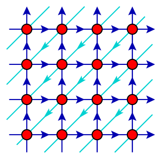
Figure 3: The two dimensional lattice preserving two exact supercharges obtained by orbifolding the eight supercharge $0+1$ SYM theory by $(Z_{N}\times Z_{N})$. Sites correspond to vector supermultiplets transforming as $U(k)$ adjoints, dark links represent bifundamental bosonic chiral supermultiplets, while light links are bifundamental Fermi supermultiplets .

3.2 Two dimensional lattices

Mother theories with eight or sixteen supersymmetries allow for the orbifolding by a $Z_{N}\times Z_{N}$ symmetry. For these lattices we choose

$$r_{1}=(q_{1}-q_{2})\ ,\qquad r_{2}=(q_{1}-q_{3})\ .$$ (7)

Starting from the mother theory with eight supercharges, the $Z_{N}\times Z_{N}$ orbifold with the above choice for the ${\bf r}$ charges reduces the exact supersymmetries from eight to two, and results in the two dimensional lattice shown in Fig. 3. At each site one finds two real bosons and two real fermions corresponding to the vector supermultiplet in 0+1 dimensions with two supercharges; the horizontal and vertical links each represent two real bosons and two real fermions, which constitute a bosonic chiral multiplet; on the diagonal links are the final two real fermions and no bosons, which comprise a Fermi multiplet. The action (discussed in §5.1) involves both kinetic terms and superpotential terms which are triangular plaquette interactions. The point symmetry group of the action consists reflections about the diagonal axes and rotations by $\pi$; together these transformations generate the four element group $C_{2v}$. The target theory in this case, a $2+1$ dimensional SYM theory with eight supercharges, has been discussed in [36, 37].

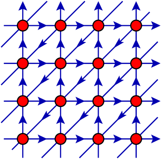
Figure 4: When the sixteen supercharge $0+1$ SYM theory is orbifolded by $(Z_{N})^{2}$, one obtains a similar lattice to that in Fig. 3, except that four supercharges are preserved, and the $\hat{x}$, $\hat{y}$ and diagonal links all correspond to identical supermultiplets, with one complex scalar and two complex one-component fermions.

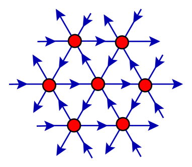
Figure 5: The lattice of Fig. 4 hides the fact that the two dimensional lattice with two exact supercharges is invariant under a $D_{6h}$ discrete symmetry preserved by the orbifold projection. It is therefore appropriate to represent the theory instead by the above hexagonal lattice.

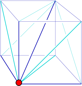
Figure 6: The sixteen supercharge $0+1$ SYM theory orbifolded by $(Z_{N})^{3}$ results in a lattice respecting two exact supercharges with the above structure. The target theory is $N=4$ SYM theory in $3+1$ dimensions. Dark blue links correspond to bosonic chiral superfields, light blue links are Fermi superfields, and a vector supermultiplet resides at each site.

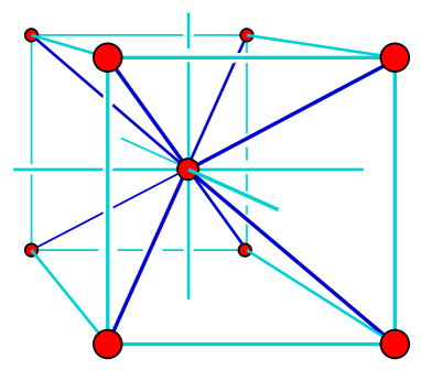
Figure 7: The lattice of Fig. 6 hides the $O_{h}$ symmetry of the action, which is better represented by the above body-centered cubic crystal. Dark lines are bosonic chiral superfields, while light lines are Fermi superfields; triangle plaquette terms appear in the superpotential (link orientation not displayed).

When the mother theory has sixteen supercharges, the lattice we obtain from the ${\bf r}$ charges Eq. (7) is shown in Fig. 5. The lattice retains four exact supercharges, there are four bosons and four real fermions at each site (a vector supermultiplet), and two real bosons and four real fermions on each link (a chiral supermultiplet). The chiral multiplets get charges $(r_{1},r_{2})$ as $(1,0),(0,1),(-1,-1)$. Thus the diagonal multiplet is also a bosonic chiral multiplet (as opposed to a Grassmann multiplet.) There is a symmetry permuting these chiral link variables, and so the symmetry group of the daughter theory is larger than it looks like in Fig. 5. Hence we draw it as an hexagonal lattice as in Fig. 5, which makes manifest the point group symmetry of the action the 12 element $D_{6}$ dihedral symmetry group. The target theory in this case, a $2+1$ dimensional field theory with sixteen supercharges, is expected to be quite interesting with an interacting superconformal phase and an enhanced $R$-symmetry related to the $SL(2,Z)$ symmetry of $N=4$ SYM in $3+1$ dimensions [35]. We discuss this lattice further in §5.2.

3.3 The three dimensional lattice

As our last example, one may orbifold the theory with sixteen supercharges by $Z_{N}^{3}$ and still retain two exact supersymmetries. The target theory in this case is $N=4$ SYM in $3+1$ dimensions. Following the prescription described above, we choose the ${\bf r}$ charges for the orbifold to be

$$r_{1}=(q_{1}-q_{2})\ ,\quad r_{2}=(q_{1}-q_{3})\ ,\quad r_{3}=(q_{1}-q_{4})\ ,$$ (8)

This orbifold condition projects the four bosonic chiral multiplets along the dark blue links of Fig 7, and three Fermi multiplets along the light blue links of Fig 7. A vector multiplet resides at each site. As in the case of the two dimensional case, the action is invariant under a larger discrete symmetry than is apparent from the lattice defined by the ${\bf r}$ vectors. This is the octahedral symmetry with inversions, the 48 element group $O_{h}$. Such a symmetry is made possible by the fact the the superdiagonal link and the cube edge links correspond to variables in the same supersymmetry multiplets. The action is more faithfully described then by the body centered cubic lattice of Fig. 7. Note that the connectivity of the two lattices is identical. The action for this lattice is discussed in §5.3.

4 The 1+1 dimensional theory with $(2,2)$ supersymmetry

A key feature in how orbifolding is able to preserve some lattice supersymmetry is the manner with which it treats gauge bosons and the associated gauginos of the target theory. Rather than having gauge fields appear as unitary matrices on links in the manner of Wilson, with gauginos represented as adjoints at the sites, the lattices discussed here have both fermion and boson bifundamental representations living on the links, making a symmetry between them possible. As a result, however, we are forced to think more carefully about the continuum limit, since the lattice spacing is no longer a parameter of the theory, but is rather dynamical, associated with the classical value of the bosonic fields about which there are quantum fluctuations.

4.1 The lattice action and continuum limit for (2,2) supersymmetry in $1+1$ dimensions

In this section we work through our simplest example, whose target theory is $(2,2)$ supersymmetric Yang-Mills theory in $1+1$ dimensions. This theory is just the dimensional reduction to $1+1$ dimensions of $N=1$ SYM theory in 3+1 dimensions, written in component fields as

$${\cal L}_{1+1}=\frac{1}{g_{2}^{2}}\mathop{\rm Tr}\left(-\frac{1}{4}F_{\mu\nu}F^{\mu\nu}+\kern 0.8pt\overline{\kern-0.8pt\Psi\kern-0.8pt}\kern 0.8pti\kern 2.5pt\raise 0.77496pt\hbox{$/$}\kern-7.5ptD\Psi+(D_{\mu}S)^{\dagger}(D^{\mu}S)+\sqrt{2}(\kern 0.8pt\overline{\kern-0.8pt\Psi\kern-0.8pt}\kern 0.8pt_{L}[S,\Psi_{R}]+h.c.)-\frac{1}{2}[S^{\dagger},S]^{2}\right)$$ (9)

where $S$ is a complex scalar and $\Psi$ is a two component Dirac fermion, each transforming as an adjoint under the $U(k)$ gauge symmetry, with gauge bosons $(v_{0},v_{1})$. Note that while $U(k)$ is not a simple group, and in principle can have two independent coupling constants, we are setting them to be equal. In the continuum, the $U(1)$ fields are all noninteracting and decouple. The apparently problematic existence of a free massless scalar in this model (the partner of the photon) will be resolved below. This is a super-renormalizable theory, which would exhibit logarithmic divergences for the scalar mass, were it not for supersymmetry which causes both the infinite and finite contributions to cancel.

The 0+1 dimensional lattice theory of Fig. 3 with two supercharges can be conveniently expressed using the superfield notation of dimensionally reduced $(0,2)$ supersymmetry in $1+1$ dimensions, as described in Appendix A. There are two types of superfields in this model: vector superfields $V$ residing at each site, containing a gauge field $v_{0}$, a complex fermion $\lambda$, a real scalar $\sigma$, and a real auxiliary field $d$; and a chiral superfield $\Phi$ on each link, consisting of a complex scalar $\phi$ and a complex fermion $\psi$. All fields are $k\times k$ matrices, with $\lambda_{n}$ and $\sigma_{n}$ transforming as adjoints under the $U(k)_{n}$ gauge symmetries, and $\phi_{n}$ and $\psi_{n}$ transforming as bifundamentals $(\raisebox{-0.5pt}{\hbox{\rule{0.4pt}{6.5pt}\hskip-0.4pt\rule{6.5pt}{0.4pt}\hskip-6.5pt\rule[6.5pt]{6.5pt}{0.4pt}}\rule[6.5pt]{0.4pt}{0.4pt}\hskip-0.4pt\rule{0.4pt}{6.5pt}},\kern 0.8pt\overline{\kern-0.8pt\raisebox{-0.5pt}{\hbox{\rule{0.4pt}{6.5pt}\hskip-0.4pt\rule{6.5pt}{0.4pt}\hskip-6.5pt\rule[6.5pt]{6.5pt}{0.4pt}}\rule[6.5pt]{0.4pt}{0.4pt}\hskip-0.4pt\rule{0.4pt}{6.5pt}}\kern-0.8pt}\kern 0.8pt)$ under the $U(k)_{n}\times U(k)_{n+1}$ gauge symmetries associated with the link ends.

In terms of these superfields, the lattice theory is given by

$$S=\frac{1}{g^{2}}\int\,dt\,\sum_{n=1}^{N}\mathop{\rm Tr}\left[\frac{1}{2}\kern 0.8pt\overline{\kern-0.8pt\Phi\kern-0.8pt}\kern 0.8pt_{n}i{\cal D}^{-}_{0}\Phi_{n}+\frac{1}{8}\kern 0.8pt\overline{\kern-0.8pt\Upsilon\kern-0.8pt}\kern 0.8pt_{n}\Upsilon_{n}\right]_{\kern 0.8pt\overline{\kern-0.8pt\theta\kern-0.8pt}\kern 0.8pt\theta}\ .$$ (10)

where $\Upsilon_{n}$ is the Grassmann chiral multiplet containing the gauge kinetic terms at site $n$. We have periodic boundary conditions with $\Upsilon_{N+1}\equiv\Upsilon_{1}$. After eliminating the auxiliary fields $d_{n}$, an expansion in terms of component fields yields

$$L=\frac{1}{g^{2}}\sum_{n}\mathop{\rm Tr} \Bigl{[} \frac{1}{2}(D_{0}\sigma_{n})^{2}+\,\kern 0.8pt\overline{\kern-0.8pt\lambda\kern-0.8pt}\kern 0.8pt_{n}\,iD_{0}\,\lambda_{n}+|D_{0}\,\phi_{n}|^{2}+\kern 0.8pt\overline{\kern-0.8pt\psi\kern-0.8pt}\kern 0.8pt_{n}\,iD_{0}\psi_{n}\Bigr{.}$$ (13)

$$-\kern 0.8pt\overline{\kern-0.8pt\lambda\kern-0.8pt}\kern 0.8pt_{n}[\sigma_{n},\lambda_{n}]+\kern 0.8pt\overline{\kern-0.8pt\psi\kern-0.8pt}\kern 0.8pt_{n}(\sigma_{n}\psi_{n}-\psi_{n}\sigma_{n+1})-\sqrt{2}\left(i\kern 0.8pt\overline{\kern-0.8pt\phi\kern-0.8pt}\kern 0.8pt_{n}(\lambda_{n}\psi_{n}+\psi_{n}\lambda_{n+1})+h.c.\right)$$

$$\left.-\left|\sigma_{n}\phi_{n}-\phi_{n}\sigma_{n+1}\right|^{2}-\frac{1}{2}\left(\phi_{n}\kern 0.8pt\overline{\kern-0.8pt\phi\kern-0.8pt}\kern 0.8pt_{n}-\kern 0.8pt\overline{\kern-0.8pt\phi\kern-0.8pt}\kern 0.8pt_{n+1}\phi_{n+1}\right)^{2}\right]\ ,$$

where

$$D_{0}\phi_{n}=\partial_{0}\phi_{n}+iv_{0,n}\phi_{n}-i\phi_{n}v_{0,n+1}$$ (14)

and similarly for $D_{0}\psi_{n}$.

The theory has a classical moduli space corresponding to all the $\phi_{n}$ being equal and diagonal, up to a gauge transformation. We now choose to expand about the point in the classical moduli space which preserves a $U(k)$ symmetry, namely

$$\phi_{n}=\frac{f}{\sqrt{2}}\times{\bf 1}_{k}\ ,$$ (15)

where ${\bf 1}_{k}$ is the $k\times k$ unit matrix and $f$ is a constant parameter with dimensions of mass. We then define a lattice spacing $a$, compactification scale $L$ and gauge coupling $g_{2}$ by

$$a\equiv\frac{1}{f}\ ,\qquad L\equiv Na\ ,\qquad g_{2}^{2}\equiv ag^{2}\ .$$ (16)

The target theory is obtained by taking the continuum limit $a\to 0$ and $N\to\infty$ for fixed $L^{2}g_{2}^{2}$, such that the dimensionless quantity $a^{2}g_{2}^{2}$ goes to zero:

$$a^{2}g_{2}^{2}=a^{3}g^{2}\to 0\ .$$ (17)

It follows that $a/L\to 0$ as well. The discrete sum $\sum_{n}$ is replaced by a spatial integral $\int\frac{{\rm d}x}{a}$, finite differences are replaced by a derivative expansion, such as

$$\phi_{n+1}(t)-\phi_{n}(t)\longrightarrow a\partial_{x}\phi(x,t)+\frac{1}{2}a^{2}\partial_{x}^{2}\phi(x,t)+\ldots\ .$$ (18)

It is convenient to write $\phi$ in terms of two hermitian fields $h_{1,2}$ as

$$\phi(x,t)=\frac{h^{(1)}(x,t)+ih^{(2)}(x,t)}{\sqrt{2}}\ .$$ (19)

Then one finds that at the classical level one obtains the target theory Eq. (9) in the continuum limit Eq. (17), after making the identifications between continuum and lattice variables

$$v_{0}=v_{0}\ ,\quad v_{1}=h^{(2)}\ ,\quad S=\frac{\sigma+ih^{(1)}}{\sqrt{2}}\ ,\quad\Psi=\begin{pmatrix}\psi\cr\kern 0.8pt\overline{\kern-0.8pt\lambda\kern-0.8pt}\kern 0.8pt\end{pmatrix}\ ,$$ (20)

where $\Psi$ is given in the Dirac basis,

$$\gamma^{0}=\begin{pmatrix}1&\ \ 0\cr 0&-1\cr\end{pmatrix}\ ,\qquad\gamma^{1}=\begin{pmatrix}0&-1\cr 1&\ \ 0\end{pmatrix}\ ,\qquad\gamma_{5}=\gamma^{0}\gamma^{1}=-\begin{pmatrix}0&\ 1\cr 1&\ 0\end{pmatrix}\ .$$ (21)

The gauge field $v_{0}$ is the same in both the lattice and the target theories. There are no unwanted fermion doublers in the spectrum; note that the $\kern 0.8pt\overline{\kern-0.8pt\phi\kern-0.8pt}\kern 0.8pt\psi\lambda$ interaction in Eq. (13) with the substitution of $\kern 0.8pt\overline{\kern-0.8pt\phi\kern-0.8pt}\kern 0.8pt\to f/\sqrt{2}$ looks like the standard kinetic term for a Wilson fermion with $r=1$.

The infinite volume limit may then be taken by sending $L^{2}g_{2}^{2}\to\infty$. In doing so, we must take care to treat separately the zeromode corresponding to shifts in the scale $f=1/a$:

$$\zeta(t)\equiv\frac{1}{\sqrt{Nk}}\sum_{n}\mathop{\rm Tr}h^{(1)}_{n}(t)\ .$$ (22)

We will refer to this mode as the “radion”, since a shift in $\zeta$ corresponds to shift in the lattice size $L$ (and the lattice spacing). With this radion mode treated separately, the infrared divergence in the propagator of the gauge singlet piece of the $S$ field in the target theory scales as $\ln L/a=\ln N$ rather than being infinite. As we will argue, so long as we specify the limits Eq. (17) such that $(ag_{2})^{2}\ln N\to 0$, this infrared divergence should be harmless (see Ref. [25] for a more detailed discussion).

The theory that results at finite lattice spacing $a$ is the target theory Eq. (9), with the addition of operators that vanish as powers of $a$. Since some of these operators do not respect the symmetries of the target theory, care must be taken to analyze renormalization as $a\to 0$. Another issue to address is the role of the radion $\zeta(t)$—it is well known that the degeneracy of a classical moduli space is lifted in quantum mechanics. For example, a classical diatomic molecule has a continuous ground state degeneracy corresponding to its angular orientation; in quantum mechanics, however, that degeneracy is lifted and the unique ground state has vanishing angular momentum, $\ell=0$. One can think of the quantum fluctuations in the molecule’s orientation as “destroying” the classical ground state. Similarly, one might well worry that fluctuations in $\zeta$ (and hence the lattice spacing) will destroy the spatial interpretation of our lattice. We will return to this worry in §4.3 and show it is unfounded, under certain restrictions on how the lattice is used.

4.2 Renormalization

We ignore the zeromode $\zeta(t)$ for the moment, and consider renormalization of the target theory as $a\to 0$. Aside from the desired operators Eq. (9), we also find at finite $a$ operators which are gauge and translational invariant, but which respect neither 1+1 dimensional Lorentz symmetry nor the enhanced $(2,2)$ supersymmetry. For example, when the fields are canonically normalized one finds the marginal operators such as

$$\mathop{\rm Tr}(\phi\partial_{1}\kern 0.8pt\overline{\kern-0.8pt\phi\kern-0.8pt}\kern 0.8pt)^{2}\ ,\qquad\mathop{\rm Tr}\kern 0.8pt\overline{\kern-0.8pt\psi\kern-0.8pt}\kern 0.8pt\partial_{1}\psi\phi\ .$$ (23)

At first sight operators like these are a disaster; however when fields are canonically normalized they have coefficients $(g_{2}a)^{2}$ and $(g_{2}a)$ respectively, and even when inserted in loops they prove to be harmless due to the exact supersymmetry of the underlying lattice.

The simplest way to analyze this theory is to maintain the noncanonical normalization used in Eq. (9), with a factor of $1/g_{2}^{2}$ in front of the effective action. At tree level and finite lattice spacing $a$, the effective action has an overall factor of $1/g_{2}^{2}$, and therefore by dimensional analysis, operators of the form $\phi^{a}\partial^{b}\psi^{2c}$ come with coefficient proportional to $a^{p-4}$, where $p=(a+b+3c)$ (here $\phi$ is a generic boson field, $\psi$ is a fermion field, and $\partial$ signifies either an $x$ or $t$ derivative anywhere in the operator). the generic form of operators with $p\leq 4$ are given in Table 2.

$p=a+b+3c$	$\phi^{a}\partial^{b}\psi^{2c}$
0	1
1	$\phi$
2	$\phi^{2}$
3	$\phi^{3}$, $\psi\psi$, $\phi\partial\phi$
4	$\phi^{4}$, $\phi\psi\psi$, $(\partial\phi)^{2}$, $\psi\partial\psi$, $\phi^{2}\partial\phi$

Table 2: Engineering dimension of operators in $d+1$ dimensions, for the field normalization that gives an overall factor $1/g^{2}$ in the action. $\phi$ and $\psi$ are generic bosons and fermions respectively; $\partial$ corresponds to a derivative.

Explicit calculation shows that at tree level all operators with $p>4$ have vanishing coefficients in the $a\to 0$ limit, while the $p=4$ operator coefficients have precisely the values of the target theory Eq. (9). Perturbative quantum effects at $\ell$ loops will generically shift the coefficient of the operator $\phi^{a}\partial^{b}\psi^{2c}$ by $a^{p-4}(ag_{2})^{2\ell}$ times possible logarithms of the form $\ln(L/a)=\ln N$. We see that only operators with $p\leq 2$ can receive divergent renormalization at one loop, and only the cosmological constant ($p=0$) can be infinitely renormalized at two loops. All higher loop graphs are finite, as befits a super-renormalizable theory. Thus for the target theory to be obtained in the $a\to 0$ limit requires that the radiative corrections which violate either $1+1$ dimensional Lorentz invariance or $(2,2)$ supersymmetry correspond only to operators with $p>2$.

Our task is then to consider the dangerous operators with $0\leq p\leq 2$ and ask whether these operators are consistent with the exact symmetries of the underlying $0+1$ dimensional lattice. if they are not, then they cannot be generated as radiative corrections in our theory. From Table 2, we see that the potentially dangerous operators are: (i) $p=0$: a cosmological constant; (ii) $p=1$: a boson tadpole $\phi$; (iii) $p=2$: a boson mass $\phi^{2}$. It is straightforward to see that in fact the symmetries of the underlying $0+1$ dimensional supersymmetric lattice forbid both the $\phi$ and the $\phi^{2}$ operators, as there are no Fermi multiplets in the spectrum, and hence no way to introduce a superpotential. However, it is possible to include a Fayet-Iliopoulos term

$$\frac{i}{g^{2}}\frac{\xi}{N}\sum_{n}\mathop{\rm Tr}\Upsilon_{n}+{\rm h.c.}$$ (24)

for the $U(1)$ field strength, the effect of which is solely to contribute to the $1+1$ dimensional theory a cosmological constant proportional to $\xi^{2}$, corresponding to the operator $1$. This term has no affect on the spectrum or interactions of the theory, and can be ignored.

We conclude that in perturbation theory, the target theory Eq. (9) is obtained, up to an uninteresting cosmological constant, without fine tuning. Given that $(ag_{2})\to 0$ in the continuum limit, the perturbative result should be reliable, with two caveats: first, the continuum limit must be taken before the large volume limit, so that the infrared $\ln N$ terms do not overwhelm suppression by powers of $ag_{2}$; and second, field values must remain small for our power counting to be valid.

The last point is cause for concern. Our power counting states that an operator of the form $\phi^{2}{\cal O}$ can generate the operator $g_{2}^{2}{\cal O}$ at one loop by connecting the $\phi$ propagators. Evidently, our power counting is equivalent to assuming that fluctuations of bosonic fields are roughly equal to $g_{2}$. Since there are zeromodes in the theory which can in principle fluctuate wildly (e.g., the radion field), we must make sure these fields do not render our analysis invalid.

4.3 The radion

We must now deal with the zeromode $\zeta(t)$ which corresponds to the classical flat direction of our scalar potential. Since the Fourier mode expansion of the link bosons is given by $\phi_{n}(t)=(f+\zeta(t)){\bf 1}+\sum_{k\neq 0}e^{ikn2\pi/N}\tilde{\phi}_{k}(t)$, where ${\bf 1}$ is the $k\times k$ unit matrix, it follows that we should replace $a\to a/(1+a\zeta(t))$ and $g_{2}^{2}\to g_{2}^{2}(1+a\zeta(t))$ through out the Lagrangian we obtain assuming $\zeta(t)=0$. In addition, there will be terms proportional to time derivatives of $\zeta(t)$. The simplest is the kinetic term

$$\frac{1}{g_{2}^{2}}\int{\rm d}t\,\int{\rm d}x\,\frac{1}{2}\,\dot{\zeta}^{2}=\frac{L}{g_{2}^{2}}\int{\rm d}t\,\frac{1}{2}\,\dot{\zeta}^{2}\ .$$ (25)

As there is no potential for $\zeta$, which behaves as a quantum mechanical variable, the ground state wave function for $\zeta$ will be uniformly spread out among all possible values for $\zeta$, which we can take to live on a compact space of size $>\frac{1}{a}$, if we consider the mother theory to derive from a compactified $N=1$ SYM in 3+1 dimensions. This would ruin our renormalization arguments of the previous section, since the argument of the previous section implies that $\zeta$ fluctuations are $O(g_{2})$ in size; if this fails to hold, we do not have any criterion for identifying an operator as irrelevant.

Note however that the kinetic term for $\zeta$ is proportional to $L$, the size of the lattice; it acts like a heavy particle for large lattices. It follows that if one performs a path integral over $\zeta$ with localized initial ($t=0$) and final ($t=T$) wave functions then $\zeta$ will remain small provided that $\Psi$ is sharply enough peaked and/or $T$ is sufficiently small compared to $L$. In particular, we can consider the Euclidean time path integral

$$Z=\int\,d\zeta_{i}\,d\zeta_{f}\,\Psi^{*}(\zeta_{f})\Psi(\zeta_{i})\int\,d\zeta(t)\,e^{-\frac{L}{g_{2}^{2}}\int_{0}^{T}\,{\rm d}t\,\frac{1}{2}\dot{\zeta}^{2}}\ ,\qquad\zeta(0)=\zeta_{i}\ ,\quad\zeta(T)=\zeta_{f}$$ (26)

where we will specify normalized Gaussian wave functions

$$\Psi(\zeta)=(\pi\zeta_{0}^{2})^{-\frac{1}{4}}e^{-\frac{\zeta^{2}}{2\zeta_{0}^{2}}}\ .$$ (27)

With this path integral, then $\zeta$ fluctuations at $t=T/2$, for example, can be computed to be

$$\frac{\langle\Psi,T|\,\zeta(T/2)^{2n}/n!\,|\Psi,0\rangle}{\langle\Psi,T|\Psi,0\rangle}=\frac{\Gamma(\textstyle{\frac{1}{2}}+n)}{\Gamma(\textstyle{\frac{1}{2}})\Gamma(1+n)}\left(\zeta_{0}^{2}+\frac{Tg_{2}^{2}}{2L}\right)^{n}\ .$$ (28)

In the above expression, the $\zeta_{0}^{2}$ corresponds to the dispersion in $\zeta$ inherent in our initial and final conditions on the path integral, while the $Tg_{2}^{2}/2L$ term corresponds to the dispersion resulting from the random walk of a free particle with mass $L/g_{2}^{2}$. However, as we discussed in the previous section, our renormalization analysis implicitly assumed that integrating out $\zeta$ (or any scalar field) at $\ell$ loops would involve the replacement in the effective action of (roughly) $\zeta\to g_{2}$. By comparing this formula with Eq. (28) above, we see that in order to justify our renormalization analysis of the previous section, we can take

$$\zeta_{0}\to 0\ ,\qquad T=L\ .$$ (29)

By taking $\zeta_{0}\to 0$, we are specifying that the initial and final conditions on the path integral are $\zeta(0)=\zeta(T)=0$. (It was convenient to perform the computation of Eq. (28) with nonzero $\zeta_{0}$, since both the denominator and the numerator on the left side of the equation vanish for $\zeta_{0}=0$). Since the volume $L=Na$ can be made arbitrarily large (so long as $(ag_{2})^{2}\ln L/a\ll 1$) our condition on $T$ poses no obstacle to taking the continuum and infinite volume limits. The main point of this analysis is that the radion behaves as a particle whose mass scales like the target theory’s volume.

The radion is not the only modulus of the theory; there exist other flat directions which generically break the $U(k)$ gauge symmetry of the target theory down to $U(1)^{k}$. The treatment of these zeromodes is the same as for the $U(k)$-singlet field $\zeta$. We have shown that it is meaningful to talk about moduli in this particular class of quantum mechanical theories, so long as we do not try to measure correlation functions over times long compared to the spatial dimensions of the lattice.

These conditions mark another departure from the usual approach to lattice field theory: all correlation functions are being measured in a particular excited state of the lattice theory, instead of the ground state of the system.

We conclude that the $1+1$ dimensional target theory with $(2,2)$ supersymmetry Eq. (9) may be obtained from our $0+1$ dimensional spatial lattice theory without any fine tuning, due to the underlying exact supersymmetry of the lattice. It would be interesting to compare lattice results for this theory with numerical results from the discrete light cone approach of ref. [38]. It should be apparent that one can generalize this model to include $SU(k)$ adjoint matter fields in the target theory, interacting via a superpotential, by adding such $SU(kN)$ adjoint matter fields to the mother theory. It is also possible to add matter fields to the target theory in the defining representation of $SU(k)$ by adding $N$ flavors of fermions to the mother theory, transforming as fundamentals of $SU(kN)$. In this case, the $Z_{N}$ used in the orbifold condition Eq. (3) would be constructed to contain contributions from the $SU(N)$ flavor symmetry of the mother theory. For the case $k=1$, resulting in an Abelian target theory, it would be interesting to see if a lattice theory could be used to explore properties of Calabi-Yau spaces, along the lines of [39].

5 Higher dimension examples

We do not discuss here the 1+1 dimensional target theories with eight or sixteen supercharges, all corresponding to the lattice of Fig. 3 with four and eight exact supersymmetries respectively. Instead, we give a brief discussion of the higher dimension theories corresponding to the lattices pictured in Figs. 3-5. A more detailed analysis is in preparation.

5.1 Eight supercharges in 2+1 dimensions

The two dimensional lattice of Fig. 3 again respects two exact supercharges. The target theory, equivalent to $N=2$ SYM reduced from $3+1$ to $2+1$ dimensions, has been discussed in refs. [36, 37]. It is a gauge theory with two complex two-component adjoint fermions, three real adjoint scalar fields, and a gauge field; all interactions are related to the gauge coupling $g_{3}$. Fig. 9 displays a single cell of our two dimensional lattice. The horizontal and vertical links are bosonic chiral superfields $\Phi_{x,y}$, while the diagonal links are Fermi superfields $X$. As discussed in the appendix, Fermi superfields $X_{a}$ in general satisfy $\kern 0.8pt\overline{\kern-0.8pt{\cal D}\kern-0.8pt}\kern 0.8ptX_{a}=E_{a}(\Phi)$, where $E_{a}(\Phi)$ is a holomorphic chiral superpotential satisfying $\kern 0.8pt\overline{\kern-0.8pt{\cal D}\kern-0.8pt}\kern 0.8ptE_{a}(\Phi)=0$. Then besides the kinetic parts of the Lagrangian for the chiral, Fermi, and vector supermultiplets ($L_{\Phi}$, $L_{X}$ and $L_{g}$ respectively), the $X_{a}$ can be coupled to a second holomorphic chiral superpotential $J^{a}(\Phi)$ satisfying $E_{a}J^{a}=0$, through a term in the Lagrangian of the form $L_{J}=\frac{1}{\sqrt{2}g^{2}}X_{a}J^{a}|_{\theta}$. Note that $E$ must be in the same representation of the gauge group as $X$, while $J$ must be in the conjugate representation.

We have drawn our lattice indicating chirality arrows for our chiral (dark blue) and Fermi (light blue) link superfields; a closed path on the lattice that consists of a single Fermi superfield link, and any number of oriented (head to tail) chiral superfield links constitutes an $E$ or a $J$ interaction—if the Fermi link is oriented in the same sense along the path as all of the chiral superfield links, then the plaquette term appears in the Lagrangian as a $J$ interaction; if the arrow of the Fermi link runs counter to the chiral superfield links in the plaquette, then that plaquette interaction arises from the $E$ superpotential. Fig. 9 makes it evident that only $J$-type interactions occur in this theory, so that $\kern 0.8pt\overline{\kern-0.8pt{\cal D}\kern-0.8pt}\kern 0.8ptX_{a}=0$ for all of the Fermi supermultiplets. Each Fermi link borders on two triangular plaquettes of opposite orientation; they are assigned a relative sign. Since the mother theory has no interactions higher than cubic in the superfields, we need only consider these three-link plaquettes as shown.

We label each site by the two-component vector ${\bf n}=\{n_{x},n_{y}\}$; $\Phi_{x}({\bf n})$ and $\Phi_{y}({\bf n})$ denote the horizontal and vertical link variables (chiral superfields) pointing outward from the site ${\bf n}$ (e.g. in the $+{\bf\hat{x}}$ and $+{\bf\hat{y}}$ directions respectively); $X({\bf n})$ is the Fermi superfield on the diagonal link pointing toward the site ${\bf n}$ (in the $-({\bf\hat{x}}+{\bf\hat{y}})$ direction). Then $L_{J}$ for this theory is given by

$$L_{J}=\frac{1}{g^{2}}\sum_{\bf n}\,\mathop{\rm Tr}\left[X({\bf n})\Bigl{(}\Phi_{x}({\bf n})\Phi_{y}({\bf n+\hat{x}})-\Phi_{y}({\bf n})\Phi_{x}({\bf n+\hat{y}})\Bigr{)}\right]{\Big{|}_{\theta}}+h.c.\ .$$ (30)

Similar to the previous example of §4, we choose to expand fields about the point in the classical moduli space $\phi_{x}({\bf n})=\phi_{y}({\bf n})=f/\sqrt{2}$ times the $k\times k$ unit matrix. It is important for our renormalization arguments that we have chosen a point in the classical moduli space that preserves the $C_{2v}$ lattice symmetry. The continuum limit is taken by taking $f=1/a$, $a\to 0$, keeping fixed $g^{2}_{3}\equiv a^{2}g^{2}$. In the continuum limit, the above interaction Eq. (30) yields the transverse kinetic term for the gauge bosons, $F_{xy}^{2}$, as well as parts of the kinetic terms for the scalars and fermions.

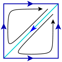
Figure 8: One cell from the lattice of Fig. 3. The black arrows indicate the plaquette terms in $L_{J}$, with opposite orientations contributing with opposite signs.

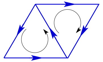
Figure 9: Two plaquettes contributing with opposite sign to the superpotential $W$ in the lattice for the target theory of sixteen supercharge SYM in $2+1$ dimensions (Fig. 5).

Analysis of the continuum limit for this theory is similar in spirit to the analysis of §4.3. Loops introduce powers of $(ag_{3}^{2})^{\ell}$, and so in principle operators with dimension $p\leq(4-\ell)$ may be renormalized at $\ell$ loops, where $p$ is given in Table 2. With the exception of the cosmological constant, which can arise as a Fayet-Iliopoulos term, none of the operators in that table with $p\leq 3$ are consistent with the underlying supersymmetry and crystal symmetry of the lattice. For example, under reflections about the diagonal axis, the have $\Phi_{x}({\bf n})\leftrightarrow\Phi_{y}(\tilde{\bf n})$ and $X({\bf n})\to-X(\tilde{\bf n})$, where $\tilde{\bf n}=\{n_{y},n_{x}\}$. This symmetry (along with the exact supersymmetry and gauge symmetry) precludes us from obtaining $\phi$, $\phi^{2}$, $\phi^{3}$ or $\phi\nabla\phi$ terms in the scalar potential. The $p=3$ operators $\phi^{*}\partial_{0}\phi$ and $\kern 0.8pt\overline{\kern-0.8pt\psi\kern-0.8pt}\kern 0.8pt\psi$ are allowed by both the crystal symmetry and supersymmetry, arising from the operator $\bigl{.}\kern 0.8pt\overline{\kern-0.8pt\Phi\kern-0.8pt}\kern 0.8pt({\bf n})\Phi({\bf n})\bigl{|}_{\kern 0.8pt\overline{\kern-0.8pt\theta\kern-0.8pt}\kern 0.8pt\theta}$, but are forbidden by time reversal symmetry. Therefore no fine tuning of the tree level theory is required to obtain the desired target theory in the continuum limit.

As in the $1+1$ dimensional case, the lattice spacing in the $2+1$ dimensional theory is dynamical and we have a radion — in fact there is one each for the horizontal and vertical link directions. In this case the inertia of each radion scales as $N^{2}$, the volume of the target theory. The treatment of the radion is as in the lower dimension theory, §4.3.

5.2 Sixteen supercharges in 2+1 dimensions

The action corresponding to the hexagonal lattice of Fig. 5 possesses an exact $D_{6}$ symmetry and four exact supercharges. The notation for this theory is similar to the familiar $N=1$ supersymmetry in $3+1$ dimensions, which also has four supercharges. The three link variables emanating from each site are described by chiral superfields $\Phi_{i}$, $i=1,2,3$, each containing a complex scalar and two complex fermions, which can be thought of as the dimensionally reduced chiral superfield from an $N=1$, $3+1$-dimensional theory. Vector superfields $V$ reside at each site, containing a real gauge field $v_{0}$, three real scalars, and two complex fermions — the dimensional reduction of a four dimensional gauge field and a Weyl fermion gaugino. There exists a superpotential $W$ which contains the triangular plaquette terms, signed according to orientation. We can define three lattice vectors

$${{\bf m}_{1}}=(1,0)\ ,\quad{\bf m}_{2}=\left(-\frac{1}{2},\frac{\sqrt{3}}{2}\right)\ ,\quad{\bf m}_{3}=\left(-\frac{1}{2},-\frac{\sqrt{3}}{2}\right)\ ,$$ (31)

and by $\Phi_{i}({\bf n})$ denote the chiral superfields leaving site ${\bf n}$ along the ${\bf m}_{i}$ direction. We can write the superpotential $W$ in terms of these fields as

$$W=\sum_{\bf n}\,\mathop{\rm Tr}\Phi_{2}({\bf n})\left(\Phi_{3}({\bf n}+{\bf m}_{2})\Phi_{1}({\bf n}-{\bf m}_{1})-\Phi_{1}({\bf n}+{\bf m}_{2})\Phi_{3}({\bf n}-{\bf m}_{3})\right)$$ (32)

corresponding to plaquettes of Fig. 9.

We expand this theory about $\phi_{i}=\frac{f}{\sqrt{2}}$ times the $k\times k$ unit matrix, where now $f$ is related to the lattice spacing $a$ as $f=\sqrt{3/2}/a$. The gauge coupling is defined again as $g_{3}^{2}\equiv a^{2}g^{2}$, and it is held fixed in the $a\to 0$ and $N\to\infty$ limits. As in the previous example of a target theory in $2+1$ dimensions with eight supercharges, there are no $p\leq 3$ operators from Table 2 that can be induced as counterterms in the continuum limit, other than a cosmological constant. Therefore one may expect to obtain the desired supersymmetric target theory without any fine tuning.

5.3 Sixteen supercharges in 3+1 dimensions: the BCC lattice

The three dimensional lattice of Fig. 7 is our third example respecting two exact supercharges. This model is of particular interest because the target theory is $N=4$ SYM with a $U(k)$ gauge group in 3+1 dimensions. This target theory can be written in $N=1$ notation in terms of three $k\times k$ chiral superfields $\Phi_{i}$ transforming as $\Phi_{i}\to U^{\dagger}\Phi_{i}U$ under the $U(k)$ gauge symmetry. These fields interact via a superpotential $W=i\epsilon_{ijk}\mathop{\rm Tr}\Phi_{i}\Phi_{j}\Phi_{k}$, as well as through gauge interactions.

Similar to the 2+1 dimensional example discussed above, the lattice theory consists of vector, chiral and Fermi supermultiplets. A new feature of the $3+1$ dimensional lattice is that there exist both $E$- and $J$-type plaquette terms. Each Fermi multiplet forms one edge of four triangular plaquettes, as shown in Fig. 10. Two of the four plaquettes run in the direction of the Fermi multiplet orientation, and are therefore of the $J$-type discussed previously; the other two run in a sense counter to the Fermi link’s orientation and form the $E$-type interactions. Each $E$- and $J$-type plaquette comes in two opposite orientations, and therefore the two contributions of each type will have a relative minus sign. The discrete symmetries of the lattice ($e.g.$ the $C_{4}$ symmetry evident in Fig. 10 ensure that the $E$ and $J$ superpotentials have the same form and strength. All superpotentials we write down have the form of a product of two chiral superfields and one Fermi superfield, corresponding to the three edges of the plaquette.

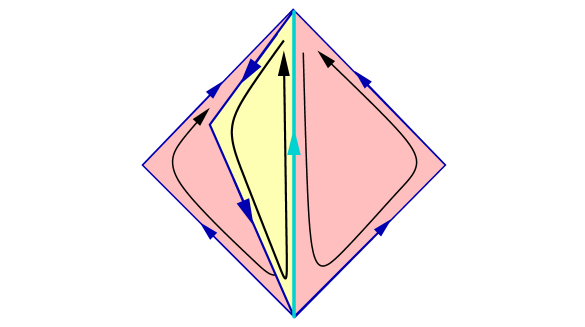
Figure 10: Each Fermi supermultiplet (light blue link) in the body centered cubic crystal of Fig. 7 forms the edge of four triangular plaquettes: one of each orientation of both the $E$ (pink) and $J$ (yellow) types.

To write down the Lagrangian, we denote each lattice site in the body centered cubic crystal by a three dimensional dimensionless vector ${\bf n}$, where we take the edge of the cell in Fig. 7 to be of coordinate length 1. Each site is associated with three Fermi multiplet links pointing outward in the ${\bf\hat{x}}$, ${\bf\hat{y}}$, and ${\bf\hat{z}}$ directions, and are denoted by $X_{a}({\bf n})$ respectively, where $a=1,2,3$. Each site is also associated with four bosonic chiral superfield links, $\Phi_{\mu}$, $\mu=0,\ldots,3$, oriented outward from the site in the four directions

$${\bf m}_{0}=\left(\textstyle{\frac{1}{2}},\textstyle{\frac{1}{2}},\textstyle{\frac{1}{2}}\right)\ ,\quad{\bf m}_{1}=\left(\textstyle{\frac{1}{2}},-\textstyle{\frac{1}{2}},-\textstyle{\frac{1}{2}}\right)\ ,\quad{\bf m}_{2}=\left(-\textstyle{\frac{1}{2}},\textstyle{\frac{1}{2}},-\textstyle{\frac{1}{2}}\right)\ ,\quad{\bf m}_{3}=\left(-\textstyle{\frac{1}{2}},-\textstyle{\frac{1}{2}},\textstyle{\frac{1}{2}}\right)\ .$$ (33)

Then for each site ${\bf n}$, we construct the six superpotentials $E_{a}$ and $J_{a}$, each with two terms of opposite sign, corresponding to the twelve triangular plaquettes associated with that site:

$$E_{a}({\bf n}) = \sqrt{2}\,\delta_{ja}\left(\Phi_{0}({\bf n})\Phi_{j}({\bf n}+{\bf m}_{0})-\Phi_{j}({\bf n})\Phi_{0}({\bf n}+{\bf m}_{j})\right)\ ,$$ (34)

$$J^{a}({\bf n}) = \sqrt{2}\,\epsilon_{ija}\left(\Phi_{i}({\bf n}+{\bf\hat{r}_{a}})\Phi_{j}({\bf n}-{\bf m}_{j})\right)\ .$$ (36)

where ${\bf\hat{r}_{a}}$ equals ${\bf\hat{x}}$, ${\bf\hat{y}}$ or ${\bf\hat{z}\,}$ for $a=1,2,3$. For example, defining ${\bf\hat{z}\,}$ to point in the vertical direction, and ${\bf m}_{3}$ and ${\bf m}_{0}$ lie in the plane of this page, the two $\Phi$ bilinears in $E_{3}$ correspond to the dark pink triangular plaquettes in Fig. 10, while the two $\Phi$ bilinears in $J^{3}$ correspond to the two light yellow plaquettes, one of which is hidden in the figure. It is not hard to show from Eq. (36) that $\mathop{\rm Tr}E_{a}J^{a}=0$ as required by supersymmetry, by considering all contributions to any particular ordering of the $\Phi$ fields ($e.g.$, $\mathop{\rm Tr}\Phi_{0}\Phi_{1}\Phi_{2}\Phi_{3}$), making use of the invariance of the lattice under translation by the ${\bf m}$ vectors and identities such as ${\bf m}_{2}+{\bf m}_{3}=-{\bf\hat{x}}$.

To create the necessary hopping terms to generate the extra dimensions, we again choose a point in the classical moduli space which preserves the $O_{h}$ lattice symmetry, namely $\Phi_{\mu}=f/\sqrt{2}$ times the $k\times k$ unit matrix, where $f=1/a$, $a$ being the lattice spacing. As before, there will be radion zeromodes associated with fluctuations of the lattice spacings, which must be fixed in the path integral as in §4.3. The continuum limit involves taking $a\to 0$ keeping the four dimensional gauge coupling $(g_{4})^{2}=a^{3}g^{2}$ fixed. At tree level one can show that indeed one obtains the target theory of $N=4$ SYM in $3+1$ dimensions. Defining the matrix $m_{\mu\nu}$, where $\mu,\,\nu=0,\ldots,3$ as

$$m_{\mu\nu}=\frac{1}{2}\begin{pmatrix}\ \ 1&\ \ 1&\ \ 1&\ \ 1\cr\ \ 1&\ \ 1&-1&-1\cr\ \ 1&-1&\ \ 1&-1\cr\ \ 1&-1&-1&\ \ 1\end{pmatrix}$$ (37)

we can express the three gauge fields $v_{1\ldots 3}$ and six real scalar fields $s_{1\ldots 6}$ of the continuum $N=4$ SYM theory as

$$\frac{s_{i}+iv_{i}}{\sqrt{2}}=m_{i\mu}\phi_{\mu}\ ,\qquad\frac{s_{4}+is_{5}}{\sqrt{2}}=m_{0\mu}\phi_{\mu}\ ,\qquad s_{6}=\sigma\ .$$ (38)

The $F_{ij}^{2}$ kinetic terms for the $v_{i}$ arise from $V_{E}+V_{J}$; the $F_{0i}^{2}$ kinetic terms come from the $|D_{0}\phi_{\mu}|^{2}$ operators in $L_{\Phi}$. The spatial parts of the kinetic terms for the $s_{1\ldots 5}$ scalars arise from $V_{d}$ and $(V_{E}+V_{J})$, with unwanted Lorentz violating contributions canceling between the two. The field $s_{6}$ develops a hopping term from the $|[\sigma,\phi]|^{2}$ operator in $L_{\Phi}$. In a similar manner it is possible to construct the four Weyl fermions of the continuum theory from the eight single component fields $\lambda$, $\chi_{i}$, and $\psi_{\mu}$. There are no unwanted doublers in our formulation.

Renormalization in this theory is trickier to analyze than in the super-renormalizable examples discussed above. Loops bring in powers of $g_{4}^{2\ell}$, and so all operators in Table 2 with $p\leq 4$ are susceptible to infinite renormalization. However, for the same reasons discussed in sections 5.1, 5.2 for the $2+1$ dimensional theories with eight and sixteen supercharges, none of the dimension $0<p\leq 3$ counterterms of Table 2 are allowable by the exact lattice symmetries. Therefore we need only consider the perturbatively marginal $p=4$ operators. To classify these $p=4$ operators which are consistent with both the underlying $O_{h}$ and supersymmetries is somewhat complicated; however it is apparent that there are now a number of allowed operators not included at tree level, which could potentially involve logarithmic fine tuning to attain the desired target theory. We have not ascertained whether fine tuning is actually necessary in this model, but will instead offer a variant of this theory which looks promising to being stable against renormalization.

5.4 Sixteen supercharges in 3+1 dimensions: the asymmetric lattice

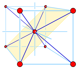
Figure 11: The two dimensional sublattice of the bcc lattice is essentially the same as the one encountered in Fig. 3, and if isolated leads to a $2+1$ dimensional continuum theory with eight supercharges, without fine tuning (see §5.1).

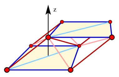
Figure 12: A redrawing of the three dimensional lattice for $N=4$ SYM in 3+1 dimensions. Dark blue and dark red links correspond to chiral supermultiplets; light blue and pink links are Fermi supermultiplet. The continuum limit is taken asymmetrically, in the horizontal planes first and subsequently in the $z$ direction. After the first limit is taken, the theory is the “linear moose” shown in Fig. 13.

It may be profitable to consider an asymmetric version of the BCC lattice of Fig. 7. Instead of choosing to take the continuum limit uniformly in each link direction, we choose instead to take the continuum limit in two dimensional planes of the lattice, and then subsequently take the continuum limit in the direction orthogonal to these planes. Note that the two dimensional sublattice lattice in these planes is essentially the same as was discussed in §5.1, as seen in Figs. 12, 12. The advantage in first taking the continuum limit in these planes is that the first step produces a family of continuum $2+1$ dimensional gauge theories with bifundamental matter fields, for which the fine tuning problems will be less serious than in $3+1$ dimensions, due to the super-renormalizability of the target theory. The subsequent continuum limit in the third spatial direction then benefits by the existence of six additional conserved supercharges which have emerged in the $2+1$ dimensional theory; these supercharges can help protect against the logarithmic fine tuning associated with dimension four operators.

Figure 13: A deconstruction of $N=4$ SYM theory in terms of a linear “moose” in $2+1$ dimensions with eight exact supersymmetries. This is the dimensional reduction of an $N=2$ SYM theory in $3+1$ dimensions with a bifundamental hypermultiplet at each link. This is the desired intermediate target theory in for the lattice in Fig. 12 after the continuum limit has been taken in the horizontal planes.

To be more specific, we propose to define the continuum limit by setting the link vevs in the horizontal plane (blue, in Fig. 12) to $\frac{f}{\sqrt{2}}$, while the links connecting the planes (red, in Fig. 12) take the value $\frac{f^{\prime}}{\sqrt{2}}$. The lattice spacings are $a_{\perp}=1/f$, $a_{\parallel}=1/f^{\prime}$. We first take the continuum limit in the horizontal planes, $a_{\perp}\to 0$, $N\to\infty$, keeping $g_{3}^{2}=g^{2}a_{\perp}^{2}$, $N^{\prime}$ and $a_{\parallel}$ fixed. The desired target theory at this stage is deconstruction [26] of $N=4$ SYM in $3+1$ dimensions in terms of a moose in $2+1$ dimensions where at each site we have a gauge theory with eight supercharges, and on each link we have a hypermultiplet, shown in Fig. 13. This hypermultiplet (we use the $3+1$ dimensional, $N=2$ language) consists the variables living on the links connecting the planes (red) in Fig. 12: four complex fermionic and two complex bosonic degrees of freedom. The second stage of our continuum limit involves taking the lattice spacing $1/f^{\prime}=a_{\parallel}\to 0$ in the $2+1$ dimensional moose.

To understand the number of parameters that need to be fine tuned in order to obtain the desired $N=4$ continuum theory from our proposed lattice, one can look at the two continuum limits separately. At the first stage we expect the lattice symmetries to forbid counterterms for dimension $p\leq 3$ operators, in a similar manner as they did for the simpler example of a $2+1$ dimensional target theory with eight supercharges discussed in 5.1. When we subsequently take the $a_{\parallel}\to 0$ limit, there is one relevant parameter to consider in the moose of Fig. 13, namely a mass term for the hypermultiplets. It seems plausible that in fact that the conformal fixed point corresponding to $N=4$ SYM in $3+1$ dimensions occurs at zero “bare” hypermultiplet mass in the moose, which would obviate fine tuning at this second stage.

We leave open the number of parameters which need to be fine tuned to obtain the $N=4$ SYM theory in $3+1$ dimensions, but we believe there is reason to be optimistic that there need be no fine tuning at all following the prescription outlined here.

6 Discussion

Motivated by deconstruction and utilizing the orbifolding techniques developed for string theory, we have shown a method for constructing supersymmetric Yang-Mills theories with extended supersymmetries on spatial lattices of various dimensions. Several of these theories — in particular, the ones with sixteen supercharges — are expected to exhibit interesting nontrivial conformal fixed points in the infrared. The basic approach relies on maintaining exactly a subset of the supersymmetries desired in the continuum limit. It is remarkable that this allows one to describe interacting scalars on the lattice without any fine tuning of parameters in the continuum limit. In fact we have argued that none of the four, eight or sixteen supercharge target theories in $1+1$ or $2+1$ dimensions require any fine tuning.

We have also given a prescription for latticizing the extremely interesting case of $N=4$ SYM in $3+1$ dimensions. We are optimistic that our proposal can be used to study this theory without any fine tuning of parameters, but this remains an open question. In any case, the degree of tuning is expected to be substantially less than by using conventional latticization approaches.

While we have focused on pure Yang-Mills theories, it is possible to generalize these theories to include matter fields as well for the target theories with four or eight supercharges. For example, in the lattice model discussed in detail for (2,2) SYM in $1+1$ dimensions, matter can be incorporated by including $N$ flavors of chiral superfields at each lattice site, and by arranging the $Z_{N}$ symmetry of the orbifold to reside in part within the $SU(N)$ flavor symmetry of the matter fields.

The theories on spatial lattices are only of limited use for numerical investigation, although one can imagine combining strong coupling expansions and large-$N$ expansions (in our notation, large-$k$ expansions) to extract information about the target theories. It is known, for example that in the large $k$ limit, the planar diagrams of the daughter theories with rescaled coupling exactly agree with those of the mother theory. For actual numerical simulation, the techniques described here can be extended to Euclidean space-time lattices. From Table 1 one sees that by reducing SYM theories down to zero dimensions, in each case the rank of the $R$ symmetry group $G_{R}$ increases by one. That means that all of the target theories discussed here can in principle be realized from pure spacetime lattices possessing half of the exact supersymmetry of the analogous spatial lattices. For example the theories with sixteen supercharges in $2+1$ and $3+1$ dimensions can be constructed from spacetime lattices possessing two or one exact real supercharges respectively. A series of papers describing such a construction are in preparation, the first of which is Ref. [25].

An open question of interest is whether one can construct lattices with enough exact supersymmetry to force the emergence of supergravity in the continuum limit.

Appendix A Superfield notation for 2 supercharges in 0+1 dimensions

In this appendix we summarize the superfield notation needed for this paper for SUSY quantum mechanics with two real supercharges. We follow the notation of ref. [39] (see also [29]) for $(0,2)$ supersymmetry in $1+1$ dimensions, which we dimensionally reduce to $0+1$ dimensions. Superspace is parametrized by a single complex Grassmann coordinate $\theta$ and its complex conjugate, $\kern 0.8pt\overline{\kern-0.8pt\theta\kern-0.8pt}\kern 0.8pt$. Superfields are functions of $t$, $\theta$ and $\kern 0.8pt\overline{\kern-0.8pt\theta\kern-0.8pt}\kern 0.8pt$. The complex supercharge $Q$ and spinor derivative $D$ are given by

$$Q=\partial_{\theta}+i\bar{\theta}\partial_{t}\ ,\qquad D=\partial_{\theta}-i\bar{\theta}\partial_{t}\ .$$ (39)

The fields we will consider are the vector, chiral, and Fermi superfield. In Wess-Zumino gauge the vector field $V$ consists of a gauge field $v_{0}$, a real scalar field $\sigma$, and a complex, one-component fermion $\chi$, and an auxiliary field $d$ (all in the adjoint representation):

$$V=(v_{0}-\sigma)-2i\theta\kern 0.8pt\overline{\kern-0.8pt\lambda\kern-0.8pt}\kern 0.8pt-2i\kern 0.8pt\overline{\kern-0.8pt\theta\kern-0.8pt}\kern 0.8pt\lambda-2\kern 0.8pt\overline{\kern-0.8pt\theta\kern-0.8pt}\kern 0.8pt\theta d\ .$$ (40)

Chiral superfields $\tilde{\Phi}$ satisfy $\kern 0.8pt\overline{\kern-0.8ptD\kern-0.8pt}\kern 0.8pt\tilde{\Phi}=0$ and have the expansion

$$\tilde{\Phi}=\phi+\sqrt{2}\,\theta\psi+i\kern 0.8pt\overline{\kern-0.8pt\theta\kern-0.8pt}\kern 0.8pt\theta\dot{\phi}$$ (41)

where $\phi$ and $\psi$ are complex boson and Grassmann fields respectively. In order to implement gauge invariance, we introduce the a gauge chiral superfield $\Psi$, which in Wess-Zumino gauge is

$$\Psi=-\kern 0.8pt\overline{\kern-0.8pt\theta\kern-0.8pt}\kern 0.8pt\theta(v_{0}+\sigma)$$ (42)

and we define the gauge covariant supersymmetric and ordinary derivatives

$${\cal D}^{+}=e^{-\Psi}De^{\Psi}\ ,\qquad{\cal D}_{0}^{-}=\partial_{t}+iV\ ,\qquad D_{0}=\partial_{t}+iv_{0}\ ,\qquad D_{0}^{\pm}=\partial_{t}+i(v_{0}\pm\sigma)\ .$$ (43)

It is convenient to define a chiral superfield $\Phi$ (no tilde) which satisfies a gauge covariant chirality condition,

$$\Phi\equiv e^{\Psi}\tilde{\Phi}=\phi+\sqrt{2}\,\theta\psi+i\kern 0.8pt\overline{\kern-0.8pt\theta\kern-0.8pt}\kern 0.8pt\theta D^{+}_{0}\phi\ ,\qquad\kern 0.8pt\overline{\kern-0.8pt{\cal D}\kern-0.8pt}\kern 0.8pt\Phi=0\ .$$ (44)

The gauge field strength is contained in the superfield $\Upsilon$ defined by

$$\Upsilon=[\kern 0.8pt\overline{\kern-0.8pt{\cal D}\kern-0.8pt}\kern 0.8pt^{+},{\cal D}^{-}_{0}]=-2\lambda+2\theta(id+D_{0}\,\sigma)-2i\kern 0.8pt\overline{\kern-0.8pt\theta\kern-0.8pt}\kern 0.8pt\theta D^{+}_{0}\,\lambda\ .$$ (45)

In addition, we must consider the so-called Fermi multiplets, Grassman superfields $X$ satisfying $\kern 0.8pt\overline{\kern-0.8pt{\cal D}\kern-0.8pt}\kern 0.8ptX=E(\Phi)$, where $E$ is a holomorphic function of chiral superfields. The new components of $X$ consist of a complex fermion $\chi$ and an auxiliary field $G$:

$$X=\chi-\sqrt{2}\,\theta G+i\kern 0.8pt\overline{\kern-0.8pt\theta\kern-0.8pt}\kern 0.8pt\theta D^{+}_{0}\chi-\sqrt{2}\,\kern 0.8pt\overline{\kern-0.8pt\theta\kern-0.8pt}\kern 0.8ptE(\Phi)$$ (46)

We normalize our fields so as to bring a common factor of $1/g^{2}$ in front of the action; all fields have canonical normalization for $g=1$. The Lagrangian for superfields $\Phi_{j}$ and $X_{\alpha}$ (where $j$ and $\alpha$ signify flavors) is then comprised of several terms:

$$L_{g} = \frac{1}{8g^{2}}\mathop{\rm Tr}\kern 0.8pt\overline{\kern-0.8pt\Upsilon\kern-0.8pt}\kern 0.8pt\Upsilon\Bigr{|}_{\kern 0.8pt\overline{\kern-0.8pt\theta\kern-0.8pt}\kern 0.8pt\theta}$$ (47)

$$= \frac{1}{g^{2}}\mathop{\rm Tr}\left(\frac{1}{2}(D_{0}\,\sigma)^{2}+\,\kern 0.8pt\overline{\kern-0.8pt\lambda\kern-0.8pt}\kern 0.8pt\,iD^{+}_{0}\,\lambda+\frac{1}{2}d^{2}\right)\ ,$$ (48)

$$L_{\Phi} = \frac{i}{2g^{2}}\sum_{j}\left(\kern 0.8pt\overline{\kern-0.8pt\Phi\kern-0.8pt}\kern 0.8pt_{j}{\cal D}^{-}_{0}\Phi_{j}\right)_{\kern 0.8pt\overline{\kern-0.8pt\theta\kern-0.8pt}\kern 0.8pt\theta}$$ (50)

$$= \frac{1}{g^{2}}\sum_{j}\left(|D_{0}\phi_{j}|^{2}-\left|\sigma\phi_{j}\right|^{2}+i\kern 0.8pt\overline{\kern-0.8pt\psi\kern-0.8pt}\kern 0.8pt_{j}D_{0}^{-}\psi_{j}+\kern 0.8pt\overline{\kern-0.8pt\phi\kern-0.8pt}\kern 0.8pt_{j}d\phi_{j}-\sqrt{2}(i\kern 0.8pt\overline{\kern-0.8pt\phi\kern-0.8pt}\kern 0.8pt_{j}\lambda\psi_{j}+h.c.)\right)$$ (51)

$$L_{X} = \frac{1}{2g^{2}}\sum_{\alpha}\left(\kern 0.8pt\overline{\kern-0.8ptX\kern-0.8pt}\kern 0.8pt^{\alpha}X_{\alpha}\right)_{\kern 0.8pt\overline{\kern-0.8pt\theta\kern-0.8pt}\kern 0.8pt\theta}$$ (53)

$$= \frac{1}{g^{2}}\sum_{\alpha}\left(i\kern 0.8pt\overline{\kern-0.8pt\chi\kern-0.8pt}\kern 0.8pt_{\alpha}D_{0}^{+}\chi_{\alpha}+|G_{\alpha}|^{2}-|E_{\alpha}(\phi)|^{2}-\sum_{j}\left[\kern 0.8pt\overline{\kern-0.8pt\chi\kern-0.8pt}\kern 0.8pt^{\alpha}\frac{\partial E_{\alpha}}{\partial\phi_{j}}\psi_{j}+h.c.\right]\right)$$ (54)

In the above expressions $(\ldots)_{\kern 0.8pt\overline{\kern-0.8pt\theta\kern-0.8pt}\kern 0.8pt\theta}$ signifies taking the coefficient of $\kern 0.8pt\overline{\kern-0.8pt\theta\kern-0.8pt}\kern 0.8pt\theta$ from the superfield in the parentheses. Further interactions can be included through a second holomorphic potential $J^{\alpha}(\Phi)$ which satisfies $\sum_{\alpha}E_{\alpha}J^{\alpha}=0$:

$$L_{J}=\frac{1}{\sqrt{2}\,g^{2}}\sum_{\alpha}\left(X_{\alpha}J^{\alpha}(\Phi)\right)_{\theta}+h.c.=-\frac{1}{g^{2}}\sum_{\alpha}\left(G_{\alpha}J^{\alpha}(\phi)+\sum_{j}\chi_{\alpha}\frac{\partial J^{\alpha}(\phi)}{\partial\phi_{j}}\psi_{j}\right)+h.c.$$ (55)

Both $d$ and $G_{\alpha}$ are auxiliary fields; integrating them out yields the scalar potential:

$$V(\phi_{j})=V_{d}+V_{G}+V_{E}=\frac{1}{2g^{2}}\sum_{a}\left(\sum_{j}\kern 0.8pt\overline{\kern-0.8pt\phi\kern-0.8pt}\kern 0.8pt_{j}T_{a}\phi_{j}\right)^{2}+\frac{1}{g^{2}}\sum_{\alpha}\left(\left|E_{\alpha}(\phi)\right|^{2}+\left|J^{\alpha}(\phi)\right|^{2}\right)$$ (56)

References

- [1] P. H. Dondi and H. Nicolai, Lattice supersymmetry, Nuovo Cim. A41 (1977) 1.
- [2] T. Banks and P. Windey, Supersymmetric lattice theories, Nucl. Phys. B198 (1982) 226–236.
- [3] S. Elitzur, E. Rabinovici, and A. Schwimmer, Supersymmetric models on the lattice, Phys. Lett. B119 (1982) 165.
- [4] J. Bartels and J. B. Bronzan, Supersymmetry on a lattice, Phys. Rev. D28 (1983) 818.
- [5] M. F. L. Golterman and D. N. Petcher, A local interactive lattice model with supersymmetry, Nucl. Phys. B319 (1989) 307–341.
- [6] P. Y. Huet, R. Narayanan, and H. Neuberger, Overlap formulation of majorana–weyl fermions, Phys. Lett. B380 (1996) 291–295, [hep-th/9602176].
- [7] I. Montvay, An algorithm for gluinos on the lattice, Nucl. Phys. B466 (1996) 259–284, [http://arXiv.org/abs/hep-lat/9510042].
- [8] J. Nishimura, Four-dimensional n = 1 supersymmetric yang-mills theory on the lattice without fine-tuning, Phys. Lett. B406 (1997) 215–218, [http://arXiv.org/abs/hep-lat/9701013].
- [9] H. Neuberger, Vector like gauge theories with almost massless fermions on the lattice, Phys. Rev. D57 (1998) 5417–5433, [http://arXiv.org/abs/hep-lat/9710089].
- [10] J. Nishimura, Applications of the overlap formalism to super yang-mills theories, Nucl. Phys. Proc. Suppl. 63 (1998) 721–723, [http://arXiv.org/abs/hep-lat/9709112].
- [11] W. Bietenholz, Exact supersymmetry on the lattice, Mod. Phys. Lett. A14 (1999) 51–62, [http://arXiv.org/abs/hep-lat/9807010].
- [12] D. B. Kaplan and M. Schmaltz, Supersymmetric yang-mills theories from domain wall fermions, Chin. J. Phys. 38 (2000) 543–550, [http://arXiv.org/abs/hep-lat/0002030].
- [13] G. T. Fleming, J. B. Kogut, and P. M. Vranas, Super yang-mills on the lattice with domain wall fermions, Phys. Rev. D64 (2001) 034510, [http://arXiv.org/abs/hep-lat/0008009].
- [14] G. T. Fleming, Lattice supersymmetry with domain wall fermions, Int. J. Mod. Phys. A16S1C (2001) 1207–1209, [http://arXiv.org/abs/hep-lat/0012016].
- [15] DESY-Munster-Roma Collaboration, F. Farchioni et. al., The supersymmetric ward identities on the lattice, Eur. Phys. J. C23 (2002) 719–734, [http://arXiv.org/abs/hep-lat/0111008].
- [16] S. Catterall and S. Karamov, A two-dimensional lattice model with exact supersymmetry, Nucl. Phys. Proc. Suppl. 106 (2002) 935–937, [http://arXiv.org/abs/hep-lat/0110071].
- [17] S. Catterall and S. Karamov, Exact lattice supersymmetry: the two-dimensional n=2 wess- zumino model, http://arXiv.org/abs/hep-lat/0108024.
- [18] K. Fujikawa, Supersymmetry on the lattice and the leibniz rule, http://arXiv.org/abs/hep-th/0205095.
- [19] I. Montvay, Supersymmetric yang-mills theory on the lattice, Int. J. Mod. Phys. A17 (2002) 2377–2412, [http://arXiv.org/abs/hep-lat/0112007].
- [20] D. B. Kaplan, Dynamical generation of supersymmetry, Phys. Lett. B136 (1984) 162.
- [21] R. Narayanan and H. Neuberger, A construction of lattice chiral gauge theories, Nucl. Phys. B443 (1995) 305–385, [http://arXiv.org/abs/hep-th/9411108].
- [22] D. B. Kaplan, A method for simulating chiral fermions on the lattice, Phys. Lett. B288 (1992) 342–347, [http://arXiv.org/abs/hep-lat/9206013].
- [23] D. B. Kaplan, Chiral fermions on the lattice, Nucl. Phys. Proc. Suppl. 30 (1993) 597–600.
- [24] H. Neuberger, Exactly massless quarks on the lattice, Phys. Lett. B417 (1998) 141–144, [http://arXiv.org/abs/hep-lat/9707022].
- [25] A. G. Cohen, D. B. Kaplan, E. Katz, and M. Unsal, Supersymmetry on a euclidean spacetime lattice. 1: A target theory with four supercharges, hep-lat/0302017.
- [26] N. Arkani-Hamed, A. G. Cohen, and H. Georgi, (de)constructing dimensions, Phys. Rev. Lett. 86 (2001) 4757–4761, [http://arXiv.org/abs/hep-th/0104005].
- [27] C. Csaki, J. Erlich, C. Grojean, and G. D. Kribs, 4d constructions of supersymmetric extra dimensions and gaugino mediation, Phys. Rev. D65 (2002) 015003, [http://arXiv.org/abs/hep-ph/0106044].
- [28] N. Arkani-Hamed, A. G. Cohen, D. B. Kaplan, A. Karch, and L. Motl, Deconstructing (2,0) and little string theories, http://arXiv.org/abs/hep-th/0110146.
- [29] H. Garcia-Compean and A. M. Uranga, Brane box realization of chiral gauge theories in two dimensions, Nucl. Phys. B539 (1999) 329–366, [http://arXiv.org/abs/hep-th/9806177].
- [30] M. R. Douglas and G. W. Moore, D-branes, quivers, and ale instantons, http://arXiv.org/abs/hep-th/9603167.
- [31] S. Kachru and E. Silverstein, 4d conformal theories and strings on orbifolds, Phys. Rev. Lett. 80 (1998) 4855–4858, [http://arXiv.org/abs/hep-th/9802183].
- [32] M. Schmaltz, Duality of non-supersymmetric large n gauge theories, Phys. Rev. D59 (1999) 105018, [http://arXiv.org/abs/hep-th/9805218].
- [33] M. J. Strassler, On methods for extracting exact non-perturbative results in non-supersymmetric gauge theories, http://arXiv.org/abs/hep-th/0104032.
- [34] I. Rothstein and W. Skiba, Mother moose: Generating extra dimensions from simple groups at large n, Phys. Rev. D65 (2002) 065002, [http://arXiv.org/abs/hep-th/0109175].
- [35] N. Seiberg, Notes on theories with 16 supercharges, Nucl. Phys. Proc. Suppl. 67 (1998) 158–171, [http://arXiv.org/abs/hep-th/9705117].
- [36] N. Seiberg, Ir dynamics on branes and space-time geometry, Phys. Lett. B384 (1996) 81–85, [http://arXiv.org/abs/hep-th/9606017].
- [37] N. Seiberg and E. Witten, The d1/d5 system and singular cft, JHEP 04 (1999) 017, [http://arXiv.org/abs/hep-th/9903224].
- [38] F. Antonuccio, O. Lunin, and S. Pinsky, Non-perturbative spectrum of two dimensional (1,1) super yang-mills at finite and large n, Phys. Rev. D58 (1998) 085009, [http://arXiv.org/abs/hep-th/9803170].
- [39] E. Witten, Phases of n = 2 theories in two dimensions, Nucl. Phys. B403 (1993) 159–222, [http://arXiv.org/abs/hep-th/9301042].