Moments of Isovector Quark Distributions from Lattice QCD

Abstract

We present a complete analysis of the chiral extrapolation of lattice moments of all twist-2 isovector quark distributions, including corrections from $N\pi$ and $\Delta\pi$ loops. Even though the $\Delta$ resonance formally gives rise to higher order non-analytic structure, the coefficients of the higher order terms for the helicity and transversity moments are large and cancel much of the curvature generated by the wave function renormalization. The net effect is that, whereas the unpolarized moments exhibit considerable curvature, the polarized moments show little deviation from linearity as the chiral limit is approached.

I Introduction

Resolving the quark and gluon structure of the nucleon remains one of the central challenges in strong interaction physics Thomas:kw . Information about the nucleon’s internal structure is parameterized in the form of leading twist parton distribution functions (PDFs), which are interpreted as probability distributions for finding specific partons (quarks, antiquarks, gluons) in the nucleon in the infinite momentum frame. PDFs have been measured in a variety of high energy processes ranging from deep-inelastic lepton scattering to Drell-Yan and massive vector boson production in hadron–hadron collisions. A wealth of experimental information now exists on spin-averaged PDFs, and an increasing amount of data is being accumulated on spin-dependent PDFs DATAREVIEW .

The fact that such a vast array of high energy data can be analyzed in terms of a universal set of PDFs stems from the factorization property of high energy scattering processes, in which the short and long distance components of scattering amplitudes can be separated according to a well-defined procedure. Factorization theorems allow a given differential cross section, or structure function, $F$, to be written (as a function of the light-cone momentum fraction $x$ at a scale $Q^{2}$) in terms of a convolution of hard, perturbatively calculable coefficient functions, $C_{i}$, with the PDFs, $f_{i}$, describing the soft, non-perturbative physics FACT_THMS :

$$F(x,Q^{2}) = \sum_{i}\int dz\ C_{i}(x/z,Q^{2}/\mu^{2},\alpha_{s}(\mu^{2}))\ f_{i}(z,\alpha_{s}(\mu^{2}))\ ,$$ (1)

where $\mu$ is the factorization scale. The coefficient functions are scale and process dependent, while the PDFs are process independent, and hence can be used to parameterize a wide variety of high energy data.

Because the PDFs cannot be calculated within perturbative QCD, the approach commonly used in global analyses of high energy data is to simply parameterize the PDFs, without attempting to assess their dynamical origin CTEQ ; MRS ; GRV ; BB . Once fitted at a particular scale, they can be evolved to any other scale through the DGLAP $Q^{2}$-evolution equations DGLAP . The focus in this approach is not so much on understanding the non-perturbative (confinement) physics responsible for the specific features of the PDFs, but rather on understanding the higher order QCD corrections for high energy processes.

In a more ambitious approach one would like to extract information about non-perturbative hadron structure from the PDFs. However, without an analytic solution of QCD in the low energy realm one must rely to varying degrees on models of (or approximations to) QCD within which to interpret the data. An extensive phenomenology has been developed over the years within studies of QCD-motivated models, and in some cases remarkable predictions have been made from the insight gained into the non-perturbative structure of the nucleon. An example is the $\bar{d}-\bar{u}$ asymmetry, predicted AWT83 on the basis of the nucleon’s pion cloud EARLY , which has been spectacularly confirmed in recent experiments at CERN, Fermilab and DESY EXPT . Other predictions, such as asymmetries between strange and anti-strange STRANGE , and spin-dependent sea quark distributions, $\Delta\bar{u}-\Delta\bar{d}$ POLSEA , still await definitive experimental confirmation. Note that none of these could be anticipated without insight into the non-perturbative structure of QCD.

Despite the phenomenological successes in correlating deep-inelastic and other high energy data with low energy hadron structure, the ad hoc nature of some of the assumptions made in deriving the low energy models from QCD leaves open questions about the ability to reliably assign systematic errors to the model predictions. One approach in which structure functions can be studied systematically from first principles, and which at the same time allows one to search for and identify the relevant low energy QCD degrees of freedom, is lattice QCD.

Lattice QCD is rapidly developing into an extremely useful and practical tool with which to study hadronic structure KFLIU . There, the equations of motion are solved numerically by discretizing space-time into a lattice, with quarks occupying the lattice sites and gluons represented by the links between the sites. Meaningful numerical results can be obtained by Wick rotating the QCD action into Euclidean space. However, because the leading twist PDFs are light-cone correlation functions (involving currents with space-time separation, $z^{2}-(ct)^{2}\approx 0$), it is, in practice, not possible to calculate PDFs directly in Euclidean space — in this case a null vector would require each space-time component to approach zero. Instead, one uses the operator product expansion to formally express the moments of the PDFs in terms of hadronic matrix elements of local operators, which can then be calculated numerically.

In relating the lattice moments to experiment, a number of extrapolations must be performed. Since lattice calculations are performed at some finite lattice spacing, $a$, the results must be extrapolated to the continuum limit, $a\to 0$, which can be done by calculating at two or more values of $a$. Furthermore, finite volume effects associated with the size of the lattice must be controlled — working with a volume that is too small can result in the omission of important physics, arising from the long-range part of the nucleon wave function. Finally, since current lattice simulations typically use quark masses $m_{q}^{\rm latt}$ above 30 MeV, an extrapolation to physical masses, $m_{q}^{\rm phys}\approx 5$ MeV, is necessary. Earlier work on moments of spin-averaged PDFs Detmold:2001jb ; Detmold:2001dv found that whereas the lattice calculations yielded results typically 50% larger than experiment when extrapolated linearly to $m_{q}^{\rm phys}$, inclusion of the nonlinear, non-analytic dependence on $m_{q}$ arising from the long range structure of the nucleon removes most of the discrepancy.

In this paper we extend the analysis to the polarized sector, which is important for several reasons. Firstly, for many years lattice calculations of the axial vector charge, $g_{A}$, have tended to lie 10% or more below the experimental value determined from neutron $\beta$ decay. Since this represents one of the benchmark calculations in lattice QCD, it is vital that the source of this discrepancy be identified. A preliminary analysis of the effects of chiral loops found WDThesis ; CHINA that the inclusion of the leading non-analytic (LNA) behavior associated with $\pi N$ intermediate states in the extrapolation of $g_{A}$ to $m_{q}^{\rm phys}$ decreased the value of $g_{A}$, thereby making the disagreement worse. On the other hand, one knows that the $\Delta$ resonance plays an important role in hadronic physics, so a more thorough investigation of its effects on spin-dependent PDFs is necessary before definitive conclusions can be drawn. Indeed, we find that although the $\Delta$ contributions formally enter at higher order in $m_{\pi}$, the coefficients of these next-to-leading non-analytic terms are large, and their effects cannot be ignored in any quantitative analysis. In addition, since there are currently no data at all on the transversity distribution in the nucleon, lattice calculations of several low transversity moments provide predictions which can be tested by future measurements. In order to make these predictions reliable, it is essential that the lattice calculations be reanalyzed to take into account the chiral corrections entering extrapolations to $m_{q}^{\rm phys}$.

The remainder of this manuscript is structured in the following manner. In Section II we describe the calculations of the moments of PDFs from matrix elements of local operators, and summarize the details of extant lattice calculations. In Section III we first examine the constraints from chiral perturbation theory and the heavy quark limit on the behavior of the moments of the various distributions as a function of the quark mass. The importance of higher order terms in the chiral expansion is then investigated within a model which preserves the non-analytic behavior of chiral perturbation theory. This information is used to construct effective parameterizations of the quark mass dependence of these moments, which are then used to extrapolate the available lattice data in Section IV. Finally, in Section V we discuss the results of this analysis and draw conclusions.

II Lattice Moments of Parton Distribution Functions

II.1 Definitions

The moments of the spin-independent, $q=q^{\uparrow}+q^{\downarrow}$, helicity, $\Delta q=q^{\uparrow}-q^{\downarrow}$, and transversity, $\delta q=q^{\top}-q^{\perp}$, distributions are defined as:

$$\langle x^{n}\rangle_{q} = \int_{0}^{1}dx\,x^{n}\ [q(x)-(-1)^{n}\bar{q}(x)]\ ,$$ (2a)

$$\langle x^{n}\rangle_{\Delta q} = \int_{0}^{1}dx\,x^{n}\ [\Delta q(x)+(-1)^{n}\Delta\bar{q}(x)]\ ,$$ (2b)

$$\langle x^{n}\rangle_{\delta q} = \int_{0}^{1}dx\,x^{n}\ [\delta q(x)-(-1)^{n}\delta\bar{q}(x)]\,,$$ (2c)

where $q^{\uparrow(\downarrow)}$ corresponds to quarks with helicity aligned (anti-aligned) with that of a longitudinally polarized target, and $q^{\top(\perp)}$ corresponds to quarks with spin aligned (anti-aligned) with that of transversely polarized target. At leading twist, these moments depend on ground state nucleon matrix elements of the operators

$${\cal O}^{\mu_{1}\ldots\mu_{n}}_{q} = i^{n-1}\ \overline{\psi}\ \gamma^{\{\mu_{1}}\,D^{\mu_{2}}\cdots\,D^{\mu_{n}\}}\psi\,,$$ (3a)

$${\cal O}^{\mu_{1}\ldots\mu_{n}}_{\Delta q} = i^{n-1}\ \overline{\psi}\ \gamma^{\{\mu_{1}}\,\gamma_{5}\,D^{\mu_{2}}\cdots\,D^{\mu_{n}\}}\psi\,,$$ (3b)

$${\cal O}^{\alpha\mu_{1}\ldots\mu_{n}}_{\delta q} = i^{n-1}\ \overline{\psi}\ \sigma^{\alpha\{\mu_{1}}\,\gamma_{5}\,D^{\mu_{2}}\cdots\,D^{\mu_{n}\}}\psi\,,$$ (3c)

respectively. Thus, for a nucleon of mass $M$, momentum $P$, and spin $S$, one has:

$$\langle P,S|{\cal O}^{\mu_{1}\ldots\mu_{n}}_{q}|P,S\rangle = 2\ \langle x^{n-1}\rangle_{q}\ P^{\{\mu_{1}}\cdots P^{\mu_{n}\}}-\text{traces}\,,$$ (4a)

$$\langle P,S|{\cal O}^{\mu_{1}\ldots\mu_{n}}_{\Delta q}|P,S\rangle = 2\ \langle x^{n-1}\rangle_{\Delta q}\ M\ S^{\{\mu_{1}}P^{\mu_{2}}\cdots P^{\mu_{n}\}}-\text{traces}\,,$$ (4b)

$$\langle P,S|{\cal O}^{\alpha\mu_{1}\ldots\mu_{n}}_{\delta q}|P,S\rangle = 2\ \langle x^{n-1}\rangle_{\delta q}\ M\ S^{[\alpha}P^{\{\mu_{1}]}P^{\mu_{2}}\cdots P^{\mu_{n}\}}-\text{traces}\,,$$ (4c)

where the braces, { $\cdots$ } ([ $\cdots$ ]), imply symmetrization (anti-symmetrization) of indices, and the ‘traces’ (containing contractions $g^{\mu_{i}\mu_{j}}$, etc.) are subtracted to make the matrix elements traceless in order that they transform irreducibly. At higher twist (suppressed by powers of $1/Q^{2}$), more complicated operators involving both quark and gluon fields contribute.

II.2 Lattice Operators

The construction of the relations (4) between moments of PDFs and matrix elements of local operators relies on the symmetry group of the Euclidean space in which one works. When formulated on a discrete space-time lattice, the symmetry group is reduced and the discretized implementation of these operators introduces several technical complications.

The discrete nature of the lattice topology means that the symmetry group of the Euclidean continuum, the orthogonal group O(4), is broken to its hyper-cubic subgroup, H(4) (the group of 192 discrete rotations which map the lattice onto itself) DolgovThesis . Unfortunately, operators in irreducible representations of O(4) may transform reducibly under H(4) and this may result in mixing with operators from lower dimensional multiplets under renormalization. Consequently, care must be exercised in the choice of operators on the lattice. For example, the continuum operator ${\cal O}^{\mu\nu}_{q}$, which corresponds to the momentum carried by quarks, can be represented on the lattice by either ${\cal O}_{q}^{(a)}=\overline{\psi}\gamma^{\{1}D^{4\}}\psi$ (belonging to a ${\bf 6}$ representation) or ${\cal O}_{q}^{(b)}=\overline{\psi}\gamma^{4}D^{4}\psi-\frac{1}{3}\sum_{i=1}^{3}\overline{\psi}\gamma^{i}D^{i}\psi$ (belonging to a ${\bf 3}$ representation). This may be regarded as an advantage since in the $a\to 0$ limit these operators are identical and any difference at non-zero lattice spacing allows for an estimate of the remaining finite size lattice artifacts to be made. In practice, this is currently somewhat ambitious, as the operator ${\cal O}_{q}^{(a)}$ requires that the hadron source should have non-zero momentum components, which leads to a statistically less well determined result. Consequently, for the operator ${\cal O}^{\mu\nu}_{q}$ we retain only the data corresponding to ${\cal O}_{q}^{(b)}$. The operators associated with the unpolarized $n=2$ and 3 moments are given by ${\cal O}_{q}^{\{114\}}-\frac{1}{2}\sum_{i=2}^{3}{\cal O}_{q}^{\{ii4\}}$ and ${\cal O}_{q}^{\{1144\}}+{\cal O}_{q}^{\{2233\}}-{\cal O}_{q}^{\{1133\}}-{\cal O}_{q}^{\{2244\}}$, respectively.

For the spin-dependent moments, the operator corresponding to the axial charge is given by ${\cal O}_{\Delta q}^{3}=\overline{\psi}\gamma^{5}\gamma^{3}\psi$. However, for the $n=1$ moment one can have on the lattice either ${\cal O}_{\Delta q}^{(a)}=\overline{\psi}\gamma^{5}\gamma^{\{1}D^{3\}}\psi$ or ${\cal O}_{\Delta q}^{(b)}=\overline{\psi}\gamma^{5}\gamma^{\{3}D^{4\}}\psi$. Once again, since the operator ${\cal O}_{\Delta q}^{(a)}$ requires non-zero momentum, we shall keep only the data corresponding to the better determined ${\cal O}_{\Delta q}^{(b)}$ operator. The operators required to calculate other moments in Eqs. (2) are described in Ref. Dolgov:2002zm .

For spin greater than 3, there are no unique, irreducible representations in H(4) for the twist-2 operators. This means that the operators for moments $n>3$ will inevitably mix with lower dimensional (or lower spin) operators. To unambiguously extract information about these moments, one would need to consider all representations for a given spin, and, with sufficiently accurate data, deduce the matrix elements of the high spin operators from the low spin operators with which they mix. Because of these difficulties, all lattice calculations have so far been restricted to moments with $n\leq 3$. Nevertheless, some features of the PDFs can be reasonably reconstructed from just the lowest few moments, as described in Ref. Detmold:2001dv .

Further subtleties arise when we consider the non-perturbative renormalization of these operators and their matching to other renormalization schemes. An operator, ${\cal O}_{\rm latt}(a)$, calculated using the lattice regularization scheme, is connected to other schemes, for example $\overline{\rm MS}$, by a renormalization factor:

$${\cal O}_{\overline{\rm MS}}(\mu)=Z_{\cal O}(\mu,a)\ {\cal O}_{\rm latt}(a)\ ,$$

where $\mu$ is the renormalization scale. To provide results in standard schemes, the renormalization functions, $Z_{\cal O}$, must therefore be calculated for each operator used. While this is done perturbatively in most calculations, non-perturbative determinations now exist Gockeler:1998rw . In what follows, results are presented in the $\overline{\rm MS}$ scheme at a renormalization scale $\mu^{2}\approx 4$ GeV².

II.3 Lattice Calculations

The first calculations of structure functions within lattice QCD were performed in the late 1980s by Martinelli and Sachrajda. Their pioneering calculations of quark distributions of the pion Martinelli:1987zd and nucleon Martinelli:1989xs were ambitious, given the speed of the computers available at the time. More recently, various calculations of greater precision have been performed Gusken:1989ad ; Dong:1995rx ; Liu:1994ab ; Fukugita:1995fh ; Aoki:1997pi ; Gusken:1999as ; Gockeler:1996wg ; Gockeler:1997jk ; BEST ; SchierholzPC ; Dolgov:2000ca ; DolgovThesis ; Dolgov:2002zm ; Gupta:1991sn ; Sasaki:2001th ; SasakiPC . In the present analysis we will focus mainly on the more recent QCDSF Gockeler:1996wg ; Gockeler:1997jk ; BEST ; SchierholzPC and LHPC-SESAM simulations Dolgov:2000ca ; DolgovThesis ; Dolgov:2002zm . The older data sets from Gupta et al. Gupta:1991sn have large uncertainties associated with renormalization, while the statistical precision of Refs. Dong:1995rx ; Liu:1994ab is comparatively low. In addition, several groups (notably the KEK Fukugita:1995fh ; Aoki:1997pi , Riken-BNL-Columbia (RBC) Sasaki:2001th ; SasakiPC and SESAM Gusken:1999as collaborations) have put particular emphasis on the $n=0$ moments of the helicity and transversity distributions — the axial and tensor charges. The simulations have been made using various quark and gluon actions, on different lattices and at different couplings. They have been performed primarily in the quenched approximation, although more recently the LHPC Dolgov:2002zm and UKQCD/QCDSF SchierholzPC groups have begun to investigate the effects of unquenching. In Table 1 we summarize the data used here, for which PDF moments and the corresponding pion masses are published.

Before including the data sets in our analysis, we impose a simple cut to reduce finite volume effects. In lattice calculations of any observable, one must ensure that the lattice size is large enough for results not to be dependent on the (unphysical) boundary conditions. This applies particularly to calculations involving low energy states such as the nucleon where the effects of the pion cloud are known to be especially important. Being the lightest, and therefore longest range, asymptotic correlation of quarks and gluons, pions are most sensitive to the boundary conditions. To avoid these difficulties, we require that the lattice volume is large enough that a pion will fit comfortably within it without “feeling the edges of the box”. A pion of mass $m_{\pi}$ has a corresponding Compton wavelength of order $\lambda_{\pi}\sim 1/m_{\pi}$, and, to avoid interference of the pion with its periodic copies, we require that the smallest dimension of the lattice box ($L$) satisfies the constraint

$$L\,>\,4\,\lambda_{\pi}\sim\frac{4}{m_{\pi}}\ .$$ (5)

The factor of $4$ in this formula is popular DolgovThesis , although somewhat arbitrary. This argument indicates that the lowest mass data point of Ref. Gockeler:1997jk and the lightest unquenched points from Ref. Dolgov:2002zm should be excluded from the analysis.

Reference	Q/U	Quark Action	Lattice	$a$ [fm]	$m_{\pi}$ [GeV]	Moments	Symbol
QCDSF Gockeler:1996wg	Q	Wilson	$16^{3}\times 32$	0.1	0.6 – 1.0	All	$\blacktriangle$
QCDSF Gockeler:1997jk	Q	Wilson	$24^{3}\times 32$	0.1	0.35 – 0.6	All	$\blacksquare$
QCDSF BEST	Q	NPIC	$16^{3}\times 32$	0.1	0.6 – 1.0	All	$\times$
QCDSF SchierholzPC	Q	NPIC	$16^{3}\times 32$	0.1	0.65 – 1.2	$\langle 1\rangle_{\Delta q}$, $\langle x^{2}\rangle_{\Delta q}$	$\blacklozenge$
	Q	NPIC	$24^{3}\times 48$	0.075	0.7 – 1.2	$\langle 1\rangle_{\Delta q}$, $\langle x^{2}\rangle_{\Delta q}$	$\bullet$
	Q	NPIC	$32^{3}\times 48$	0.05	0.6 – 1.25	$\langle 1\rangle_{\Delta q}$, $\langle x^{2}\rangle_{\Delta q}$	$\times+$
MIT Dolgov:2002zm	Q	Wilson	$16^{3}\times 32$	0.1	0.58 – 0.82	All	$\bigstar$
MIT-SESAM Dolgov:2002zm	U	Wilson	$16^{3}\times 32$	0.1	0.63 – 1.0	All	$\lozenge$
MIT-SCRI Dolgov:2002zm	U	Wilson	$16^{3}\times 32$	0.1	0.48 – 0.67	All	$\square$
KEK Fukugita:1995fh ; Aoki:1997pi	Q	Wilson	$16^{3}\times 20$	0.14	0.52 – 0.97	$\langle 1\rangle_{\Delta q}$, $\langle 1\rangle_{\delta q}$	$\blacktriangledown$

Table 1: Simulation parameters for lattice calculations of the moments of PDFs included in our analysis. Q/U corresponds to quenched/unquenched simulations, and NPIC denotes the nonperturbatively improved clover quark action. “All” moments correspond to $\langle x^{i}\rangle_{q}$ for $i=1,2,3$, $\langle x^{i}\rangle_{\Delta q}$ for $i=0,1,2$, and $\langle x^{i}\rangle_{\delta q}$ for $i=0,1$. The symbols shown in the final column correspond to those plotted in Figs. 8, 9 and 10.

In terms of quark flow, the evaluation of matrix elements of the operators in Eqs. (3) includes both connected and disconnected diagrams, corresponding to operator insertions in quark lines which are connected or disconnected (except through gluon lines) with the nucleon source — see Fig. 1.

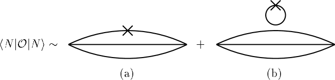
Figure 1: Connected (a) and disconnected (b) contributions to the matrix elements of an operator (indicated by the cross). Such diagrams occur in quenched QCD as well as in full QCD.

Since the numerical computation of disconnected diagrams is considerably more difficult, only exploratory studies of these have thus far been completed Gusken:1999as , and the data analyzed here include only connected contributions. However, because the disconnected contributions are flavor independent (for equal $u$ and $d$ quark masses), they exactly cancel in the difference of $u$ and $d$ moments. Therefore, until more complete lattice simulations become available, one can only compare lattice moments of the flavor non-singlet $u-d$ distribution with moments of phenomenological PDFs CTEQ ; MRS ; GRV .

Whilst the chiral behavior of quenched QCD is different from that of full QCD Chen:2001gr , in the region where current lattice data from both quenched and unquenched simulations are available, the differences are well within the statistical errors, indicating that internal quark loops do not play a significant role over this mass range. As calculations begin to probe lighter quark masses, the differences should become more apparent and it will become necessary to analyze quenched and unquenched data separately Young:2001nc . Until the differences become statistically distinguishable, however, we shall combine the data from the two sets of simulations.

III Chiral Behavior of PDF Moments

To compare the lattice results with the experimentally measured moments, one must extrapolate the data from the lowest quark mass used ($\sim 50$ MeV) to the physical value ($\sim$ 5 MeV). This is commonly done by assuming that the moments depend linearly on the quark mass. However, as discussed in Ref. Detmold:2001jb , such a linear extrapolation overestimates the experimental values of the unpolarized isovector moments CTEQ ; MRS ; GRV by some 50% in all cases. Since the discrepancy persists in unquenched simulations Dolgov:2000ca ; DolgovThesis ; Dolgov:2002zm , it suggests that important physics is being omitted from either the lattice calculations or their extrapolations. In Refs. Detmold:2001jb ; Detmold:2001dv the chiral behavior of the moments of the unpolarized isovector distributions was found to be vital in resolving this discrepancy. Here we summarize the results of the earlier unpolarized study, and extend the analysis to the moments of the spin-dependent isovector distributions in the nucleon.

III.1 Chiral Symmetry and Leading Non-analytic Behavior

The spontaneous breaking of the chiral SU_L(N_f)$\times$SU_R(N_f) symmetry of QCD generates the nearly massless Goldstone bosons (pions), whose importance in hadron structure is well documented. At small pion masses, hadronic observables can be systematically expanded in a series in $m_{\pi}$ — chiral perturbation theory ($\chi$PT) CHIPT . The expansion coefficients are generally free parameters, determined from phenomenology. One of the unique consequences of pion loops, however, is the appearance of non-analytic behavior in the quark mass. From the Gell-Mann–Oakes–Renner relation one finds that $m_{\pi}^{2}\sim m_{q}$ at small $m_{\pi}$, so that terms involving odd powers or logarithms of $m_{\pi}$ are non-analytic functions of the quark mass. Their presence can lead to highly nonlinear behavior near the chiral limit ($m_{\pi}\to 0$) Detmold:2001hq . Because the non-analytic terms arise from the infrared behavior of the chiral loops, they are generally model independent.

The leading order (in $m_{\pi}$) non-analytic term in the expansion of the moments of PDFs was shown in Ref. TMS to have the generic behavior $m_{\pi}^{2}\log m_{\pi}$ arising from $\pi N$ intermediate states. This was later confirmed in $\chi$PT CHPT , where the coefficients of these terms were also calculated. In Ref. Detmold:2001jb a low order chiral expansion for the moments of the non-singlet distribution, $u-d$, was developed, incorporating the LNA behavior of the moments as a function of $m_{q}$ and also connecting to the heavy quark limit (in which quark distributions become $\delta$-functions centered at $x=1/3$) Detmold:2001dv . For the moments of the unpolarized isovector distribution, these considerations lead to the following functional form for the moments Detmold:2001dv :

$$\langle x^{n}\rangle_{u-d}\ =\ a_{n}\left(1+c_{\rm LNA}m_{\pi}^{2}\log\frac{m_{\pi}^{2}}{m_{\pi}^{2}+\mu^{2}}\right)\ +\ b_{n}\frac{m_{\pi}^{2}}{m_{\pi}^{2}+m_{b,n}^{2}}\ ,$$ (6)

where (for $n>0$) the chiral coefficient $c_{\rm LNA}=-(1+3g_{A}^{2})/(4\pi f_{\pi})^{2}$ CHPT , and $b_{n}$ is a constant constrained by the heavy quark limit:

$$b_{n}=\frac{1}{3^{n}}-a_{n}\left(1-\mu^{2}c_{\rm LNA}\right)\ .$$ (7)

The $n=0$ moment, which corresponds to isospin charge, is not renormalized by pion loops. The parameter $\mu$ is introduced to suppress the rapid variation of the logarithm for pion masses away from the chiral limit where $\chi$PT breaks down. Physically it is related to the size of the nucleon core, which acts as the source of the pion field Detmold:2001hq . Finally, the fits to the data are quite insensitive to the choice of $m_{b,n}$ (as long as it is large), and it has been set to 5 GeV for all $n$ Detmold:2001dv .

A similar analysis leads to analogous lowest order LNA parameterizations of the mass dependence of the spin-dependent moments CHINA :

$$\langle x^{n}\rangle_{\Delta u-\Delta d}\ =\Delta a_{n}\left(1+\Delta c_{\rm LNA}m_{\pi}^{2}\log\frac{m_{\pi}^{2}}{m_{\pi}^{2}+\mu^{2}}\right)\ +\ \Delta b_{n}\frac{m_{\pi}^{2}}{m_{\pi}^{2}+m_{b,n}^{2}}\,,$$ (8)

and

$$\langle x^{n}\rangle_{\delta u-\delta d}\ =\delta a_{n}\left(1+\delta c_{\rm LNA}m_{\pi}^{2}\log\frac{m_{\pi}^{2}}{m_{\pi}^{2}+\mu^{2}}\right)\ +\ \delta b_{n}\frac{m_{\pi}^{2}}{m_{\pi}^{2}+m_{b,n}^{2}}\,,$$ (9)

where the LNA coefficients are given by $\Delta c_{\rm LNA}=-(1+2g_{A}^{2})/(4\pi f_{\pi})^{2}$ and $\delta c_{\rm LNA}=-(1+4g_{A}^{2})/[2(4\pi f_{\pi})^{2}]$ CHPT . In the heavy quark limit, both $\Delta u(x)-\Delta d(x)$ and $\delta u(x)-\delta d(x)$ are given by $\frac{5}{3}\delta(x-1/3)$ Gockeler:1996bm , which leads to the constraints:

$$\Delta b_{n}=\frac{5}{3^{n+1}}-\Delta a_{n}\left(1-\mu^{2}\Delta c_{\rm LNA}\right)\,,$$ (10)

and

$$\delta b_{n}=\frac{5}{3^{n+1}}-\delta a_{n}\left(1-\mu^{2}\delta c_{\rm LNA}\right)\,.$$ (11)

These are the most general lowest order parameterizations of the twist-2 PDF moments consistent with chiral symmetry and the heavy quark limits of QCD.

III.2 Phenomenological Constraints

In Refs. Detmold:2001jb ; Detmold:2001dv we presented analyses of unpolarized data based on Eq. (6), where it was concluded that current lattice data alone do not sufficiently constrain the extrapolation of these moments, and more accurate data at smaller quark masses ($m_{q}\lesssim 15-20$ MeV) are required to determine the parameter $\mu$. In that work, a central value of $\mu=500$ MeV (550 MeV when the heavy quark limit was not included Detmold:2001jb ) was chosen as it best reproduced both the lattice data and the phenomenological values at the physical point. However, the systematic error on this parameter is very large; indeed, the raw lattice data are consistent with $\mu=0$ (a linear extrapolation).

In order to make the phenomenological constraint of $\mu$ more quantitative, we employ the following measure of the goodness of fit of the extrapolated values (at $m_{\pi}^{\rm phys}$) of the first three non-trivial unpolarized moments to the phenomenological values, $\langle x^{i}\rangle_{u-d}^{\rm expt}$, as a function of $\mu$:

$$\chi(\mu)=\sum_{i=1}^{3}\frac{(\langle x^{i}(\mu)\rangle_{u-d}-\langle x^{i}\rangle_{u-d}^{\rm expt})^{2}}{(\langle x^{i}\rangle_{u-d}^{\rm expt})^{2}}\,.$$ (12)

Figure 2: The goodness of fit of the extrapolated values of the first three non-trivial moments to the phenomenological values as a function of $\mu$ calculated using Eq. (12).

We assume that both the lattice data for the unpolarized moments and their extrapolation based on Eq. (6) are correct, and use the phenomenological values for these moments as a constraint.

The behavior of the function $\chi(\mu)$ is shown in Fig. 2, and the best value of $\mu$ is indeed found to be 500 MeV. This value is also comparable to the scale at which the behavior found in other observables, such as magnetic moments and masses, switches from smooth and constituent quark-like (slowly varying with respect to the current quark mass) to rapidly varying and dominated by Goldstone boson loops. For fits to lattice data on hadron masses, Leinweber et al. found values in the range 450 to 660 MeV MASS when a sharp momentum cut-off was used. The similarity of these scales for the various observables is not coincidental, but simply reflects the common scale at which the Compton wavelength of the pion becomes comparable to the size of the bare nucleon. The value of $\mu$ is also similar to the scale predicted by the $\chi^{2}$ fits to the model discussed in the following section (see also Ref. Detmold:2001jb ).

III.3 $\Delta$ Intermediate States

When we come to the calculation of polarized PDFs, there is considerable phenomenological evidence to suggest that the $\Delta$ resonance will play an important role. Within the cloudy bag model (CBM), a convergent perturbative expansion of the physical nucleon, in terms of the number of virtual pions, required the explicit inclusion of the $\Delta$-isobar Dodd:1981ve ; Thomas:1982kv — see also Ref. Oettel:2002cw for a recent, fully relativistic investigation. Without the $\Delta$, the ratio of the bare to renormalized pion-nucleon coupling constant was found to be very large (as in the old Chew-Wick model). With it, they typically agree to within 10-15%. The essential physics is that the vertex renormalization associated with coupling to the $\Delta$ or to an $N$–$\Delta$ transition compensates almost exactly for the reduction caused by wave function renormalization. Of course, the same mechanisms apply to the renormalization of the axial charge, $g_{A}$, as to the pion nucleon coupling, $g_{\pi NN}$.

In the limit that the $\Delta$ is degenerate with the nucleon, $\Delta M\equiv M_{\Delta}-M\to 0$, the leading non-analytic contribution from the $\Delta$ is of the same order as that arising from the nucleon, namely $m_{\pi}^{2}\log m_{\pi}^{2}$. In the limit $\Delta M\to\infty$, the $\Delta$ contribution can be integrated out, and it formally does not make any non-analytic contribution. For a finite, but non-zero $\Delta M$, the vertex renormalization involving the $\Delta$ is not a leading non-analytic term, but instead enters as $m_{\pi}^{3}/\Delta M$. However, the coefficient of this next-to-leading non-analytic (NLNA) term is huge Chen:2001et — roughly three times bigger than the $m_{\pi}^{3}$ term in the expansion of the nucleon mass MASS . Faced with such a large coefficient, one cannot rely on naive ordering arguments alone to identify the important physics.

The solution adopted by Leinweber et al. MASS in the analysis of the chiral behavior of baryon masses was to calculate corrections arising from those pion loop diagrams responsible for the most rapid variation with $m_{q}$. The finite spatial extension of the pion source leads naturally to an ultraviolet cut-off at the $\pi NN$ and $\pi N\Delta$ vertices Hecht:2002ej . The parameter, $\Lambda\sim 1/R$ (with $R$ the size of the source) associated with these vertices is constrained phenomenologically. This approach ensures that the LNA and NLNA behavior of $\chi$PT is reproduced in the $m_{\pi}\to 0$ limit, while the transition to the heavy quark limit ($m_{\pi}>\Lambda$), where pion loops are suppressed as inverse powers of $m_{\pi}$, is also guaranteed. Alternatively, one can study the variation of PDF moments with $m_{\pi}$ within a model, such as the cloudy bag Thomas:1982kv ; Theberge:1981mq , which also ensures the full LNA and NLNA behavior of $\chi$PT, and in addition provides a simple physical interpretation of the short-distance contributions (in this case through the MIT bag model). Rather than rely on a specific model, in the present analysis we adopt the approach of Ref. MASS and calculate the pion loop integrals with hadronic vertices constrained phenomenologically.

The overall renormalization of the forward matrix elements of the operators of Eqs. (3) in nucleon states is then given by:

$$\langle N|{\cal O}^{\mu_{1}\ldots\mu_{n}}_{i}|N\rangle_{\rm dressed}=\frac{Z_{2}}{Z_{i}}\langle N|{\cal O}^{\mu_{1}\ldots\mu_{n}}_{i}|N\rangle_{\rm bare}\ ,\ \ \ \ i=q,\Delta q,\delta q\ ,$$ (13)

where $Z_{2}$ is the wave function renormalization constant,

$$Z_{2}^{-1}=1+Z_{2}^{N}+Z_{2}^{\Delta}\,,$$ (14)

and $Z_{i}$ are the vertex renormalization constants described below. The $N$ and $\Delta$ contributions to the wave function renormalization, illustrated in the first row of Fig. 3, are given in the heavy baryon limit by Theberge:1981mq :

$$Z_{2}^{N} = \frac{3g_{A}^{2}}{(4\pi f_{\pi})^{2}}\int_{0}^{\infty}\frac{k^{4}u^{2}(k)dk}{\omega^{3}(k)}\,,$$ (15)

$$Z_{2}^{\Delta} = \frac{4}{9}\frac{g_{\pi N\Delta}^{2}}{g_{\pi NN}^{2}}\frac{3g_{A}^{2}}{(4\pi f_{\pi})^{2}}\int_{0}^{\infty}\frac{k^{4}u^{2}(k)dk}{\omega(k)(\omega(k)+\Delta M)^{2}}\ ,$$ (16)

where $\omega(k)=\sqrt{k^{2}+m_{\pi}^{2}}$ is the pion energy, and $u(k)$ is the form factor parameterizing the momentum dependence of the $\pi NN$ and $\pi N\Delta$ vertices, for which we choose a dipole form,

$$u(k) = \frac{\Lambda^{4}}{(k^{2}+\Lambda^{2})^{2}}\ .$$ (17)

The numerical calculations are performed with a characteristic momentum cut-off scale $\Lambda=0.8$ GeV, just a little softer than the measured axial form factor of the nucleon Thomas:tv ; Guichon:1982zk – although the results are relatively insensitive to the precise value of $\Lambda$, as illustrated below. The ratio of the $\pi N\Delta$ to $\pi NN$ couplings can be determined from SU(6) symmetry ($g_{\pi N\Delta}/g_{\pi NN}=\sqrt{72/25}$), however, in the numerical calculations we consider a range of values for the ratio. SU(6) symmetry is also used to relate matrix elements of the twist-2 operators in the bare $\Delta$ and $N$-$\Delta$ transition to those in the bare nucleon. Lattice calculations of $\Delta$ or $N$-$\Delta$ transition matrix elements will in future test the reliability of this approximation.

Figure 3: Contributions to the wave function and vertex renormalization of the nucleon matrix elements of the operators ${\cal O}_{i}^{\mu_{1}\ldots\mu_{n}}$, $i=q,\Delta q,\delta q$, in Eq. (3). Solid, double and dashed lines denote nucleon, $\Delta$ and pion propagators and the crossed circle and box indicate the insertion of the relevant operators. Diagrams $Z_{2}^{N}$ and $Z_{2}^{\Delta}$ denote the contributions to wave function renormalization (a derivative with respect to the external momentum is implied).

The renormalization constants for the spin-independent, helicity and transversity operators are given by

$$Z_{q}^{-1} = 1+Z_{1,U}^{NN}+Z_{1,U}^{\Delta\Delta}+Z_{1,U}^{\rm tad}\,,$$ (18a)

$$Z_{\Delta q}^{-1} = 1+Z_{1,P}^{NN}+Z_{1,P}^{N\Delta}+Z_{1,P}^{\Delta N}+Z_{1,P}^{\Delta\Delta}+Z_{1,P}^{\rm tad}+Z_{1,P}^{N\rm WT}+Z_{1,P}^{\Delta\rm WT}\,,$$ (18b)

$$Z_{\delta q}^{-1} = 1+Z_{1,P}^{NN}+Z_{1,P}^{N\Delta}+Z_{1,P}^{\Delta N}+Z_{1,P}^{\Delta\Delta}+\frac{1}{2}Z_{1,P}^{\rm tad}+\frac{1}{2}Z_{1,P}^{N\rm WT}+\frac{1}{2}Z_{1,P}^{\Delta\rm WT}\,.$$ (18c)

The contributions from the coupling to nucleon intermediate states are given by:

$$Z_{1,U}^{NN} = -\frac{g_{A}^{2}}{(4\pi f_{\pi})^{2}}\int_{0}^{\infty}\frac{k^{4}u^{2}(k)dk}{\omega^{3}(k)}\,,$$ (19)

and

$$Z_{1,P}^{NN} = \frac{1}{3}\frac{g_{A}^{2}}{(4\pi f_{\pi})^{2}}\int_{0}^{\infty}\frac{k^{4}u^{2}(k)dk}{\omega^{3}(k)}\,,$$ (20)

for the unpolarized and polarized operators, respectively. One can explicitly verify that the LNA behavior of these contributions is $m_{\pi}^{2}\log m_{\pi}^{2}$. The $\Delta$ contributions to the unpolarized and polarized operators are equivalent,

$$Z_{1,U}^{\Delta\Delta}=Z_{1,P}^{\Delta\Delta} = \frac{20}{27}\frac{g_{\pi N\Delta}^{2}}{g_{\pi NN}^{2}}\frac{g_{A}^{2}}{(4\pi f_{\pi})^{2}}\int_{0}^{\infty}\frac{k^{4}u^{2}(k)dk}{\omega(k)(\omega(k)+\Delta M)^{2}}\ ,$$ (21)

while the $N\Delta$ transition contributes only to the spin-dependent operators,

$$Z_{1,P}^{\Delta N}=Z_{1,P}^{N\Delta} = \frac{16}{27}\frac{g_{\pi N\Delta}^{2}}{g_{\pi NN}^{2}}\frac{g_{A}^{2}}{(4\pi f_{\pi})^{2}}\int_{0}^{\infty}\frac{k^{4}u^{2}(k)dk}{\omega^{2}(k)(\omega(k)+\Delta M)}\ .$$ (22)

These contributions are illustrated in the middle row in Fig. 3. Expanding these terms for small $m_{\pi}$, one finds that the leading non-analytic terms associated with the $\Delta$ and $N$–$\Delta$ transition contributions enter at orders $m_{\pi}^{4}\log m_{\pi}^{2}$ and $m_{\pi}^{3}$, respectively. The contributions from the tadpole diagrams, which are independent of $g_{A}$, are also identical for the unpolarized and polarized cases, and given by

$$Z_{1,U}^{\rm tad}\ =\ Z_{1,P}^{\rm tad} = -\frac{2}{(4\pi f_{\pi})^{2}}\int_{0}^{\infty}\frac{k^{3}u^{2}(k)dk}{\omega^{2}(k)}\ .$$ (23)

The tadpole contributions also enter at order $m_{\pi}^{2}\log m_{\pi}^{2}$ CHPT , as can be verified directly from Eq. (23).

While the inclusion of the $\Delta$ resonance is important for quantitative descriptions of baryon structure, we also know from phenomenological studies that the higher order (in $m_{\pi}$) Weinberg-Tomozawa contact term Weinberg:1966fm ; Tomozawa:1966gg plays a vital role in low energy $S$-wave pion–nucleon scattering Thomas:1981ps . Because of the Adler-Weisberger relation AW between $\pi N$ cross sections and $g_{A}$, any term which affects $\pi N$ cross sections should also have some effect on $g_{A}$ Morgan:1985kr . In fact, within the CBM Morgan et al. Morgan:1985kr found that this term largely resolves the discrepancy between the bag model value of $g_{A}=1.09$ and the empirical value of $g_{A}$ for bag radii $R\in(0.9,1.1)$ fm. In the present treatment, since we do not use the CBM explicitly, but rather parameterize the pion source via the phenomenological form factor $u(k)$, we determine the overall strength of the Weinberg-Tomozawa term so as to reproduce the contribution found in the CBM, as outlined in Ref. Morgan:1985kr . The relative contributions of the diagrams with $N$ and $\Delta$ intermediate states, however, illustrated in the last row of Fig. 3, can be fixed by SU(6) symmetry. These contributions to the operator renormalization can then be written:

$$Z_{1,P}^{N\rm WT} = C_{WT}\int_{0}^{\infty}\frac{k^{4}u^{2}(k)dk}{\omega^{2}(k)}\ ,$$ (24)

$$Z_{1,P}^{\Delta\rm WT} = \frac{C_{WT}}{18}(1+\sqrt{2})\frac{g_{\pi N\Delta}^{2}}{g_{\pi NN}^{2}}\int_{0}^{\infty}\frac{k^{4}u^{2}(k)dk}{\omega(k)(\omega(k)+\Delta M)}\ ,$$ (25)

for the $N$ and $\Delta$ intermediate states, respectively, where $C_{WT}$ is the overall normalization. For the above range of $R$, the physical value of $g_{A}$ can be reproduced to within a few percent for the corresponding range of $C_{WT}\in(0.21,0.30)$. In the following numerical analysis, we use this range as an estimate of the systematic error on the Weinberg-Tomozawa contribution. Even though the non-analytic behavior of the integrals in Eqs. (24) and (25) is $m_{\pi}^{3}$ or higher, their contributions are found to be significant. Note, however, that the Weinberg-Tomozawa terms contribute only to spin-dependent matrix elements, and make no contribution to unpolarized matrix elements.

With the exception of the matrix elements of the unpolarized, $n=0$ operator, the renormalization of each moment of the various distributions is independent of $n$. The $n=0$ operator, which corresponds to the isospin charge, is not renormalized — additional contributions from operator insertions on the pion propagator cancel those shown in Fig. 3.

The pion mass dependence of the various contributions to the wave function and operator renormalization is shown in Fig. 4. For the ratio of the couplings, $g_{\pi N\Delta}/g_{\pi NN}$, SU(6) symmetry is assumed. The relative size of the terms $Z_{1}^{NN}$ and $Z_{1}^{\Delta\Delta}$ in the spin-dependent and spin-independent cases already makes it clear that intermediate states involving $\Delta$ resonances are much more significant in the former case. In particular, whereas $Z_{1,P}^{NN}$ does little to counter the effect of the wave function renormalization, the $\Delta$ contributions $Z_{1,P}^{\Delta\Delta}$, $Z_{1,P}^{N\Delta}$, and $Z_{1,P}^{\Delta N}$ essentially cancel its effect.

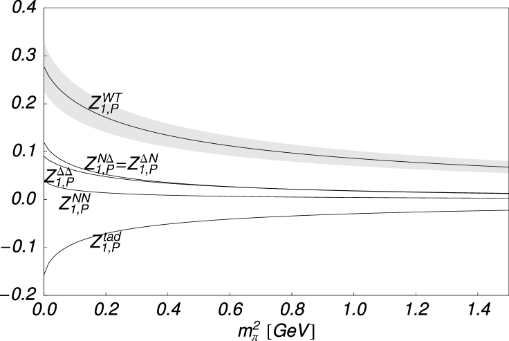
Figure 4: Contributions to the pion loop renormalization of the matrix elements of the twist–2 operators required to evaluate the moments of the PDFs. The upper panel shows nucleon wave function renormalizations ($Z_{2}^{N}$, $Z_{2}^{\Delta}$) and spin-independent operator renormalizations. The lower panel shows the contributions to the renormalization of spin-dependent operators, and the shaded region is an estimate of the uncertainty in the Weinberg–Tomozawa term, $Z^{\rm WT}_{1,P}\equiv Z^{\rm NWT}_{1,P}+Z^{\rm\Delta WT}_{1,P}$. The $g_{\pi N\Delta}/g_{\pi NN}$ coupling constant ratio is set to the SU(6) symmetric value of $\sqrt{72/25}$.

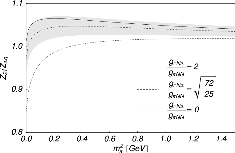
Figure 5: Pion dressing of the matrix elements of the spin-independent (upper panel) and spin-dependent (lower panel) operators in Eq. (3) for various values of the ratio of coupling constants, $g_{\pi N\Delta}/g_{\pi NN}$. The shading in the lower panel indicates the variation about the dashed curve ($g_{\pi N\Delta}/g_{\pi NN}=\sqrt{72/25}$) caused by the uncertainty in the Weinberg–Tomozawa term. The behavior of $Z_{2}/Z_{\delta q}$ is similar to that of $Z_{2}/Z_{\Delta q}$.

To explore the sensitivity of the results to the strength of the $\Delta$ contribution, in Fig. 5 we show the combined effect of the pion dressing on spin-averaged (upper panel) and spin-dependent (lower panel) nucleon matrix elements in Eq. (13) for a range of values of the ratio $g_{\pi N\Delta}/g_{\pi NN}$. For illustration we choose values of $g_{\pi N\Delta}/g_{\pi NN}$ equal to zero (no $\Delta$ states), $\sqrt{72/25}$ (SU(6) coupling) and 2 (phenomenological value needed to reproduce the width of the physical $\Delta$ resonance). In the unpolarized case, the effect of this variation is relatively small — less than 3% over the entire range of pion masses considered here. In contrast, the effect of the $\Delta$ on the helicity and transversity moments (matrix elements of the spin-dependent operators ${\cal O}_{\Delta q}^{\mu_{1}\ldots\mu_{n}}$ and ${\cal O}_{\delta q}^{\mu_{1}\ldots\mu_{n}}$) is far more significant. If the contribution from the $\Delta$ (and the $N$-$\Delta$ transition matrix elements) is ignored ($g_{\pi N\Delta}/g_{\pi NN}=0$), $\left.Z_{2}/Z_{\Delta q}\right|_{m_{\pi}^{\rm phys}}=0.90$, while including these contributions with SU(6) couplings increases this to $\left.Z_{2}/Z_{\Delta q}\right|_{m_{\pi}^{\rm phys}}=1.01$, and to $\left.Z_{2}/Z_{\Delta q}\right|_{m_{\pi}^{\rm phys}}=1.04$ at the phenomenological value $g_{\pi N\Delta}/g_{\pi NN}=2$. Consequently, when the effects of the $\Delta$ are included with a coupling constant which is consistent with phenomenology, one finds that there is almost no curvature in the extrapolation of the spin-dependent moments. This result is relatively stable against variations Thomas:tv ; Guichon:1982zk in the dipole mass parameter, $\Lambda$, in the range $\sim 0.7-1.0$ GeV — especially for the spin-dependent moments, as illustrated in Fig. 6.

Figure 6: Dependence of the renormalization of the nucleon matrix elements in Eq. (13) on the dipole mass parameter, $\Lambda$, at the physical pion mass, for the SU(6) value of $g_{\pi N\Delta}/g_{\pi NN}$.

Matrix elements of the twist-2 operators (3) in bare nucleon states will necessarily be analytic functions of the quark mass ($m_{q}\sim m_{\pi}^{2}$), so the one pion loop renormalization described above is the only possible source of LNA contributions. Consequently, the LNA behavior of the matrix elements in Eq. (13) will be given by

$$\langle{\cal O}^{\mu_{1}\ldots\mu_{n}}_{i}\rangle_{\rm LNA}=Z_{2}^{\rm LNA}-Z_{i}^{\rm LNA}\ ,\ \ \ \ \ i=q,\Delta q,\delta q\ .$$ (26)

If the $N$–$\Delta$ mass splitting is artificially reduced to zero, $\Delta$ intermediate states become degenerate with the corresponding nucleon intermediate states, and the respective $\Delta$ diagrams formally give rise to LNA contributions. Leaving the $g_{\pi N\Delta}/g_{\pi NN}$ ratio free, the coefficients of the LNA contributions (the $m_{\pi}^{2}\log m_{\pi}^{2}$ term) to the various matrix elements can then be written:

$$\langle{\cal O}^{\mu_{1}\ldots\mu_{n}}_{q}\rangle_{\rm LNA}=Z_{2}^{\rm LNA}-Z_{q}^{\rm LNA}=-\frac{1}{(4\pi f_{\pi})^{2}}\left[\left(3+\frac{16}{27}\frac{g^{2}_{\pi N\Delta}}{g^{2}_{\pi NN}}\right)g^{2}_{A}+1\right]\,,$$ (27a)

$$\langle{\cal O}^{\mu_{1}\ldots\mu_{n}}_{\Delta q}\rangle_{\rm LNA}=Z_{2}^{\rm LNA}-Z_{\Delta q}^{\rm LNA}=-\frac{1}{(4\pi f_{\pi})^{2}}\left[\left(2-\frac{4}{9}\frac{g^{2}_{\pi N\Delta}}{g^{2}_{\pi NN}}\right)g^{2}_{A}+1\right]\,,$$ (27b)

$$\langle{\cal O}^{\mu_{1}\ldots\mu_{n}}_{\delta q}\rangle_{\rm LNA}=Z_{2}^{\rm LNA}-Z_{\delta q}^{\rm LNA}=-\frac{1}{(4\pi f_{\pi})^{2}}\left[\left(2-\frac{4}{9}\frac{g^{2}_{\pi N\Delta}}{g^{2}_{\pi NN}}\right)g^{2}_{A}+\frac{1}{2}\right]\,.$$ (27c)

This makes it clear that, whereas an increase in $g_{\pi N\Delta}/g_{\pi NN}$ from $0$ (no $\Delta$ contributions) tends to increase the effective coefficient of the chiral logarithm in the unpolarized case, for the spin-dependent operators it acts to suppress it. Indeed, assuming the bare axial coupling $g_{A}=1.26$, at $g_{\pi N\Delta}/g_{\pi NN}=2.43$ the LNA coefficient for the polarized moments is zero, and for larger values it even becomes positive. Whilst this exact cancellation is an artifact of setting $\Delta M=0$, it highlights the significant role played by the $\Delta$ resonance.

From this analysis and the numerical results shown earlier, one can conclude that the inclusion of the $\Delta$ resonance will cause only a minor quantitative change in the extrapolation of unpolarized moments, and in practical extrapolations of lattice data the $\Delta$ can be neglected with no loss of accuracy, given the current uncertainties in the data. In contrast, the $\Delta$ leads to a qualitatively different picture for the extrapolation of the spin-dependent moments and must be included there.

There are a number of possible approaches that can be taken to account for the $\Delta$ contributions. One strategy would be to include the one-loop renormalizations numerically in the extrapolations, along the lines of the calculation of self-energies in the hadron mass extrapolations in Refs. MASS ; Young:2001nc . One could also replace the momentum integrals in the expressions for $Z_{1}$ and $Z_{2}$ with discrete sums over momenta which are available on the lattice, $\int d^{3}k\to(1/V)(2\pi/a)^{3}\sum_{k_{x},k_{y},k_{z}}$, where $V$ is the spatial volume of the lattice, as in the analysis of the $\rho$ meson mass in Ref. DISCRETE (see also QUENCH ). Because of the discretization of space-time on the lattice, the lattice momenta are restricted to values $k_{\mu}=2\pi n_{\mu}/aL_{\mu}$, where $L_{\mu}$ is the number of lattice sites in the $\mu$ direction and the integer $n_{\mu}$ runs between $-L_{\mu}/2$ and $+L_{\mu}/2$. We have checked that at large $m_{\pi}^{2}$ the differences between the integral and discrete sum are only a few percent or less, however, at small $m_{\pi}^{2}$ values the momentum gap between $k_{\mu}=0$ and the minimum momentum allowed, $k_{\mu}=\pm 2\pi/aL_{\mu}$, may introduce corrections.

Although this procedure is more accurate in principle, in practical extrapolations of lattice data it is not as straightforward to implement as an extrapolation formula based on a simple functional form would be. For this purpose it is more useful to preserve the simplicity of a single formula which interpolates between the distinct realms of chiral perturbation theory and contemporary lattice simulations, as proposed in Refs. Detmold:2001jb ; Detmold:2001dv . In order to test whether one can continue to apply a modified form of the extrapolation formula in Eq. (6) to lattice data for the spin-dependent moments, as well as the spin-independent, we attempt to fit the pion mass dependence of the renormalization factors shown in Fig. 5 using the form

$$Z_{2}/Z_{i}=\alpha_{i}+\beta_{i}m_{\pi}^{2}+\frac{\gamma_{i,\rm LNA}}{(4\pi f_{\pi})^{2}}m_{\pi}^{2}\log\left[\frac{m_{\pi}^{2}}{m_{\pi}^{2}+\mu_{i}^{2}}\right]\ ,\ \ \ \ \ i=q,\Delta q,\delta q\ ,$$ (28)

with $\alpha_{i}$, $\beta_{i}$ and $\mu_{i}$ treated as free parameters, but with $\gamma_{i,\rm LNA}$ fixed to the values obtained analytically in the limit $\Delta M\to 0$, as shown in Table 2. The fits to $Z_{2}/Z_{i}$ $(i=q,\Delta q,\delta q)$ are illustrated in Fig. 7 for the average of the $g_{\pi N\Delta}/g_{\pi NN}$ values from SU(6) symmetry ($\sqrt{72/25}$) and phenomenology (2). Fits for other values of the coupling are equally good. It is remarkable that the LNA form (28) is indeed able to reproduce the full calculations of $Z_{2}/Z_{i}$ with such high accuracy, given that the full calculations include higher order effects (in $m_{\pi}$) associated with the $\Delta$ and Weinberg-Tomozawa contributions. The best fit values of $\mu$, shown in Table 2, are only slightly smaller than those found in earlier work Detmold:2001jb ; Detmold:2001dv . Note that the functional form in Eq. (28) does not include the modifications designed to ensure the correct heavy quark limit, as in Eqs. (6)–(9) — incorporating this constraint leads to only marginal changes in the parameter $\mu$ Detmold:2001dv .

	$Z_{2}/Z_{q}$		$Z_{2}/Z_{\Delta q}$		$Z_{2}/Z_{\delta q}$
$g_{\pi N\Delta}/g_{\pi NN}$	$c_{\rm LNA}$	$\mu$ (GeV)	$\Delta c_{\rm LNA}$	$\mu$ (GeV)	$\delta c_{\rm LNA}$	$\mu$ (GeV)
0	$3g_{A}^{2}+1$	0.45	$2g_{A}^{2}+1$	0.28	$2g_{A}^{2}+\frac{1}{2}$	0.32
$\sqrt{\frac{72}{25}}$	$\frac{107}{25}g_{A}^{2}+1$	0.39	$\frac{18}{25}g_{A}^{2}+1$	0.25	$\frac{18}{25}g_{A}^{2}+\frac{1}{2}$	0.29
1.85	$4.51g_{A}^{2}+1$	0.38	$0.48g_{A}^{2}+1$	0.25	$0.48g_{A}^{2}+\frac{1}{2}$	0.30
2	$\frac{43}{9}g_{A}^{2}+1$	0.37	$\frac{2}{9}g_{A}^{2}+1$	0.24	$\frac{2}{9}g_{A}^{2}+\frac{1}{2}$	0.29

Table 2: Fits to the dependence on $m_{\pi}^{2}$ of the calculated renormalization factors, obtained by varying $\alpha_{i}$, $\beta_{i}$ and $\mu_{i}$ in Eq. (28). The LNA coefficients and the mass parameters $\mu_{i}$ are shown for various values of the $g_{\pi N\Delta}/g_{\pi NN}$ ratio: 0 (no $\Delta$), $\sqrt{72/25}$ (SU(6)), 2 (phenomenological value) and 1.85 (average of SU(6) and phenomenological values).

Figure 7: Fits to the calculated renormalization factors $Z_{2}/Z_{i},\ i=q,\Delta q,\delta q$, in Eq. (13) using the functional form in Eq. (28), as a function of $m_{\pi}^{2}$. The $\pi N\Delta$ to $\pi NN$ coupling ratio has been set to the average of the SU(6) and phenomenological values ($g_{\pi N\Delta}/g_{\pi NN}=1.85$), and $g_{A}$ to the tree level value, 1.26. The corresponding values of $\mu$ are given in the third row of Table 2.

As discussed above, excluding the isospin charge, all moments of each operator are renormalized in the same manner. Hence, our conclusions regarding the inclusion of the $\Delta$-isobar apply equally well to extrapolations of $g_{A}=\langle 1\rangle_{\Delta u-\Delta d}$ and all other moments of the helicity and transversity distributions.

IV Extrapolation of Lattice Data

Having established that the LNA formula, Eq. (28), provides a good approximation to the full calculation, in this section we examine the effects of extrapolating the available lattice data on the twist-2 PDF moments using the forms (6), (8) and (9), with the LNA coefficients determined in the limit $\Delta M\to 0$. Rather than show the moments versus the scale and renormalization scheme dependent quark mass, Figs. 8, 9 and 10 give the moments of the unpolarized, helicity and transversity distributions, respectively, as a function of the pion mass squared. The data have been extrapolated using a naive linear extrapolation (short-dashed lines), as well as the improved chiral extrapolations with the LNA chiral coefficients and values of $\mu$ given in Table 2, with $m_{b,n}$ fixed at 5 GeV Detmold:2001dv .

For the spin-dependent moments, four curves are shown in Figs. 9 and 10: the long-dashed curves correspond to ignoring $\Delta$ intermediate states ($g_{\pi N\Delta}=0$), while the central solid lines in each panel of the figures include the effects of the $\Delta$ with a coupling ratio $g_{\pi N\Delta}/g_{\pi NN}=1.85$ (average of SU(6) and phenomenological values) and the central value for the Weinberg-Tomozawa coefficient, $C_{WT}=0.255$. The upper and lower solid lines correspond to $g_{\pi N\Delta}/g_{\pi NN}=2$, $C_{WT}=0.30$ and $g_{\pi N\Delta}/g_{\pi NN}=\sqrt{72/25}$, $C_{WT}=0.21$, respectively. Because the effect of the $\Delta$ is almost negligible for the unpolarized moments, these curves are all essentially collinear, and for clarity only one is shown in Fig. 8. The extrapolated values are shown in Table 3, along with the associated errors (which are described in the Appendix) and the experimental values for the unpolarized and helicity moments CTEQ ; MRS ; GRV ; BB (there are currently no data for the transversity moments). Note that even though there is no curvature expected for large $m_{\pi}$, the slopes of the linear and LNA fits differ slightly at large $m_{\pi}$ values due to the constraints of the heavy quark limit incorporated into the forms (6), (8) and (9).

Moment	Value		Extrapolation errors			$a_{n},\Delta a_{n},\delta a_{n}$
	Experimental	Extrapolated	Statistical	$\Delta$, WT states	$\mu$
$\langle x\rangle_{u-d}$	0.145(4)	0.176	0.012	0.0008	0.022	0.141
$\langle x^{2}\rangle_{u-d}$	0.054(1)	0.054	0.015	0.0003	0.007	0.044
$\langle x^{3}\rangle_{u-d}$	0.022(1)	0.024	0.008	0.0001	0.003	0.019
$\langle 1\rangle_{\Delta u-\Delta d}$	1.267(4)	1.124	0.045	0.020	0.022	1.084
$\langle x\rangle_{\Delta u-\Delta d}$	0.210(25)	0.273	0.015	0.005	0.005	0.262
$\langle x^{2}\rangle_{\Delta u-\Delta d}$	0.070(11)	0.140	0.035	0.003	0.003	0.135
$\langle 1\rangle_{\delta u-\delta d}$	—	1.224	0.057	0.019	0.025	1.187
$\langle x\rangle_{\delta u-\delta d}$	—	0.506	0.089	0.008	0.010	0.490

Table 3: Values of the unpolarized, helicity and transversity moments, extrapolated to the physical pion mass using Eqs. (6), (8) and (9) and the parameters in Table 2. The experimental and systematic errors listed here are described in the Appendix. For comparison, experimental values of the moments where known (unpolarised values from moments of distributions of Refs. CTEQ ; MRS ; GRV , helicity moments from Ref. BB in scenario I (NLO)) and the best fit parameters ($a_{n}$, $\Delta a_{n}$, $\delta a_{n}$) are also listed.

With respect to the moments of the unpolarized PDFs, this analysis confirms our earlier finding that it is essential to incorporate the correct non-analytic behavior into the chiral extrapolation. When this is done, there is good agreement between the extrapolated moments at the physical pion mass and the corresponding experimental data. On the other hand, for the polarized PDFs we have the surprising result that once the $\Delta$ resonance is included, the effect of the non-analytic behavior is strongly suppressed, and a naive linear extrapolation of the moments provides quite a good approximation to the more accurate form.

Figure 8: The lowest three non-trivial moments of the unpolarized distribution $u-d$, extrapolated using a naive linear fit (dashed lines) and the improved chiral extrapolation (solid lines). The stars indicate the experimentally measured moments at the physical pion mass, and the lattice data are taken from the sources listed in Table 1, where the various plotting symbols are defined.

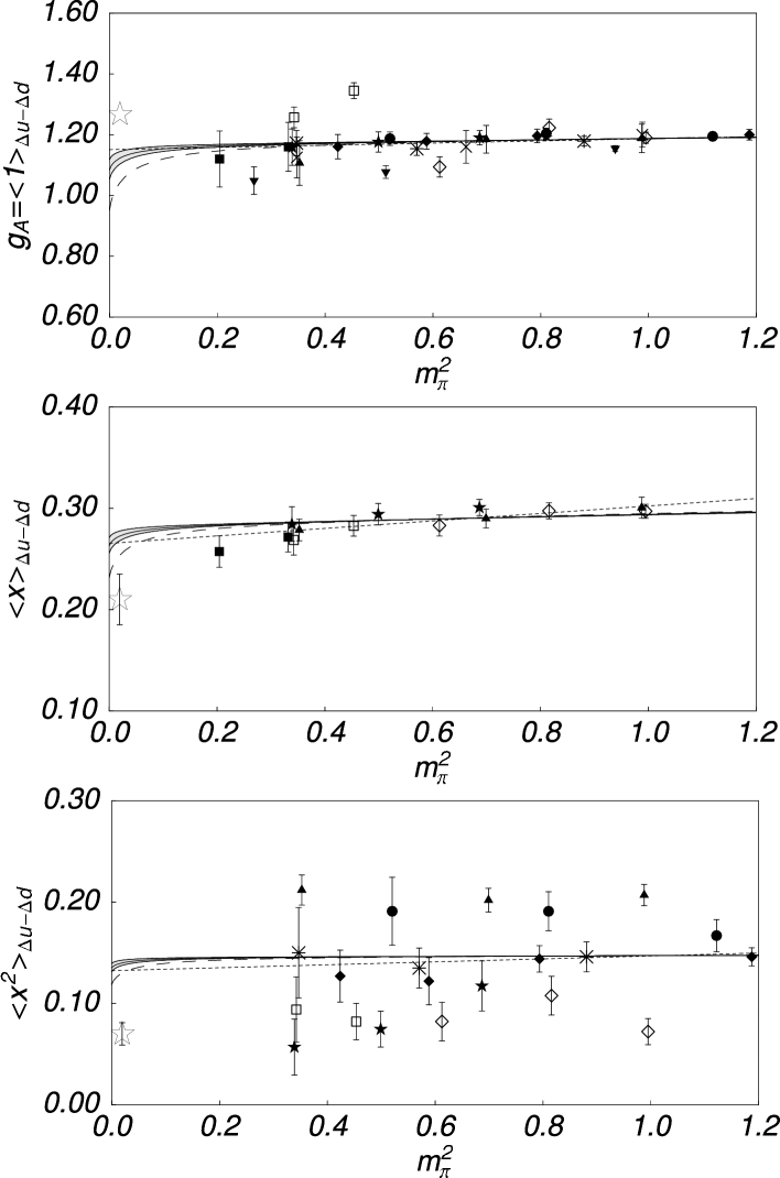
Figure 9: The lowest three moments of the helicity distribution $\Delta u-\Delta d$, extrapolated using a naive linear extrapolation (short-dashed lines) and the improved chiral extrapolation described in the text. In each panel, the long-dashed lines correspond to fits with no $\Delta$ and the LNA coefficient determined from $\chi$PT, while the solid lines are fits obtained using $g_{\pi N\Delta}/g_{\pi NN}=2$ (upper solid curves) and $\sqrt{72/25}$ (lower solid curves). The lattice data are taken from the sources listed in Table 1.

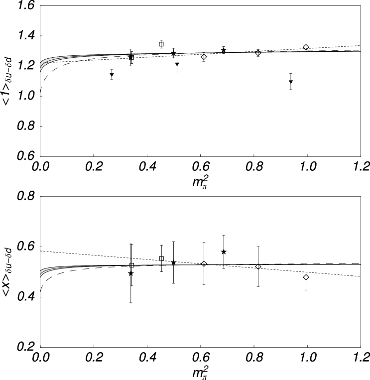
Figure 10: The lowest two moments of the transversity distribution $\delta u-\delta d$. All curves are as described in Fig. 9.

In the case of the axial charge (the $n=0$ moment of $\Delta u-\Delta d$), the extrapolated value lies some 10% below the experimental value, with an error of around 5%. However, $g_{A}$ appears to be particularly sensitive to finite volume corrections, with larger lattices tending to give larger values of $g_{A}$. Furthermore, there is some sensitivity to the choice of action — simulations with domain wall fermions (DWF), which satisfy exact chiral symmetry, are found to give larger values than those with Wilson fermions Sasaki:2001th . As almost all of the currently available lattice data are obtained from very small lattices ($L\sim 1.6$ fm), we consider the current level of agreement quite satisfactory.

Additionally, there is some uncertainty arising from the inclusion of the heavy quark limit in our fits; if this constraint is omitted, the large $m_{\pi}^{2}$ behavior of our fits coincides with the linear fits that are shown as one would expect. For $\langle x\rangle_{\delta u-\delta d}$ ($\langle x\rangle_{\Delta u-\Delta d}$), a fit ignoring the heavy quark limit gives a physical value of 0.559 (0.257) rather than 0.506 (0.273) as given in Table 3 (with a smaller effect in the other moments).

The uncertainty in the experimental determination of the higher moments of the spin-dependent PDFs is considerably larger, and from the current data one would have to conclude from Fig. 9 that the level of agreement between experiment and the extrapolated moments is acceptable. Clearly the scatter in the lattice data for the second moment means that at present we cannot have much confidence in the predicted value. We do note, in addition, that this is one case where there is a tendency for the full QCD points to lie somewhat below the quenched QCD results. It is obviously of some importance that this issue be resolved in future lattice simulations.

V Conclusion

The insights into non-perturbative hadron structure offered by the study of parton distribution functions makes this an extremely interesting research challenge. It is made even more important and timely by the tremendous new experimental possibilities opened by facilities such as HERMES, COMPASS, RHIC-Spin and Jefferson Lab. Lattice QCD offers the only practical method to actually calculate hadron properties within non-perturbative QCD, and it is therefore vital to test how well it describes existing data. Because current limitations on computer speed restrict lattice simulations to quark masses that are roughly a factor of 6 too large, one must be able to reliably extrapolate the lattice data to the physical quark (or pion) mass in order to compare with experiment.

Traditionally such extrapolations have been made using a naive linear extrapolation as a function of $m_{\pi}^{2}$ (or quark mass). In Ref. Detmold:2001jb , Detmold et al. showed that it was essential to include the leading non-analytic behavior of chiral perturbation theory in this extrapolation procedure. Only then were the existing lattice data for the moments of the unpolarized parton distribution functions in agreement with the experimental moments. Here we have confirmed this conclusion by calculating the next-to-leading non-analytic behavior within a chiral quark model, including the $\Delta$-isobar, and showing that it led to precisely the same conclusion.

We have also investigated the variation of the moments of the polarized parton distributions to next-to-leading order. In this case the inclusion of the $\Delta$-isobar makes a dramatic difference. Indeed, once the $\Delta$ is included, the helicity and transversity moments show little or no curvature as the chiral limit is approached and a naive linear extrapolation formula is reasonably accurate. In case a more accurate extrapolation procedure is desired, we propose convenient formulae which suitably build in the non-analytic behavior in both the unpolarized and the polarized cases. The value of $g_{A}$ extracted from the extrapolation procedure at the physical pion mass is within 10% of the experimental value. Given the sensitivity of this quantity to lattice volume (current simulations use quite small lattices) and quark action (domain wall fermions tend to give a larger value of $g_{A}$ than Wilson fermions), we consider this a very satisfactory result. We look forward with great anticipation to the next generation of lattice simulations of parton distribution functions at smaller quark masses and on larger volumes.

Appendix A Statistical and systematic errors

In this Appendix, we describe the estimates of the statistical and systematic errors in our fits that are presented in Table 3.

To determine an estimate of the error associated with the statistical uncertainty of the lattice data, we use the estimated standard deviation. For data, $f_{i}$, and weights, $\omega_{i}$, given at abscissae $x_{i}$ ($i=1,\ldots,n$), the estimated standard deviation of a fitting form $f(x;\vec{\alpha})$ with parameters $\vec{\alpha}$ is:

$$\sigma_{0}=\sqrt{\frac{1}{n-1}\sum_{i=1}^{n}\omega_{i}\left(f_{i}-f(x_{i};\vec{\alpha}_{0})\right)^{2}}\ ,$$ (29)

where $\vec{\alpha}_{0}$ are the best fit parameters. The statistical errors assigned to the fits are then determined by varying the fit parameters ($a_{n}$, $\Delta a_{n}$, $\delta a_{n}$) from their optimal values (given in the right-most column of Table 3) to obtain an increase of unity in the standard deviation.

In order to estimate the systematic errors arising from the form of our fits, we first consider the uncertainty in the values of $g_{\pi N\Delta}/g_{\pi NN}$ and $C_{WT}$, taking half the difference between the physical values of the moments obtained with $g_{\pi N\Delta}/g_{\pi NN}=2$, $C_{WT}=0.30$ and $g_{\pi N\Delta}/g_{\pi NN}=\sqrt{72/25}$, $C_{WT}=0.21$. We also consider the uncertainty in the fit parameter $\mu$ by taking half the difference between the physical moments obtained with $\mu$ 20% above and below the fits obtained in Table 2. The resulting systematic uncertainties are listed in Table 3.

References

- (1) A.W. Thomas and W. Weise, The Structure Of The Nucleon, (Wiley-VCH, Berlin, Germany, 2001).
- (2) M. Erdmann, Talk given at 8th International Workshop on Deep Inelastic Scattering and QCD (DIS 2000), Liverpool, England, 25-30 Apr. 2000, arXiv:hep-ex/0009009; E.W. Hughes and R. Voss, Ann. Rev. Nucl. Part. Sci. 49, 303 (1999).
- (3) J.C. Collins, D.E. Soper and G. Sterman, Nucl. Phys. B261, 104 (1985); R. Brock et al., Rev. Mod. Phys. 67, 157 (1995).
- (4) H.L. Lai et al., Eur. Phys. J. C 12, 375 (2000).
- (5) A.D. Martin, R.G. Roberts, W.J. Stirling and R.S. Thorne, Eur. Phys. J. C 14, 133 (2000).
- (6) M. Glück, E. Reya, and A. Vogt, Eur. Phys. J. C 5, 461 (1998).
- (7) J. Blümlein and H. Böttcher, arXiv:hep-ph/0203155.
- (8) Yu.L. Dokshitzer, Sov. Phys. - JETP 46, 641 (1977); V. N. Gribov and L. N. Lipatov, Sov. J. Nucl. Phys. 15, 438 (1972). L. N. Lipatov, Sov. J. Nucl. Phys. 20, 94 (1975) P. Altarelli and G. Parisi, Nucl. Phys. B126, 298 (1977).
- (9) A.W. Thomas, Phys. Lett. B 126, 97 (1983).
- (10) J.D. Sullivan, Phys. Rev. D 5, 1732 (1972); E.M. Henley and G.A. Miller, Phys. Lett. B 251, 453 (1990); A.I. Signal, A.W. Schreiber and A.W. Thomas, Mod. Phys. Lett. A 6, 271 (1991); W. Melnitchouk, A.W. Thomas and A.I. Signal, Z. Phys. A 340, 85 (1991); S. Kumano, Phys. Rev. D 43, 3067 (1991); S. Kumano and J.T. Londergan, Phys. Rev. D 44, 717 (1991); W.-Y.P. Hwang, J. Speth and G.E. Brown, Z. Phys. A 339, 383 (1991); For reviews see: J. Speth and A.W. Thomas, Adv. Nucl. Phys. 24, 83 (1998); S. Kumano, Phys. Rep. 303, 183 (1998).
- (11) P. Amaudraz et al., Phys. Rev. Lett. 66, 2712 (1991); A. Baldit et al., Phys. Lett. B 332, 244 (1994); E.A. Hawker et al., Phys. Rev. Lett. 80, 3715 (1998); K. Ackerstaff et al., Phys. Rev. Lett. 81, 5519 (1998).
- (12) A.I. Signal and A.W. Thomas, Phys. Lett. B 191, 205 (1987); X. Ji and J. Tang, Phys. Lett. B 362, 182 (1995); S.J. Brodsky and B.-Q. Ma, Phys. Lett. B 381, 317 (1996); W. Melnitchouk and M. Malheiro, Phys. Rev. C 55, 431 (1997).
- (13) A.I. Signal and A.W. Thomas, Phys. Rev. D 40, 2832 (1989); A.W. Schreiber, A.I. Signal and A.W. Thomas, Phys. Rev. D 44, 2653 (1991); D. Diakonov, V.Y. Petrov, P.V. Pobylitsa, M.V. Polyakov and C. Weiss, Phys. Rev. D 56, 4069 (1997); K. Tsushima, A.W. Thomas and G.V. Dunne, arXiv:hep-ph/0107042; R.J. Fries, A. Schafer and C. Weiss, arXiv:hep-ph/0204060.
- (14) K.F. Liu, S.J. Dong, T. Draper, D.B. Leinweber, J. Sloan, W. Wilcox and R.M. Woloshyn, Phys. Rev. D 59, 112001 (1999).
- (15) W. Detmold, W. Melnitchouk, J.W. Negele, D.B. Renner and A.W. Thomas, Phys. Rev. Lett. 87, 172001 (2001).
- (16) W. Detmold, W. Melnitchouk, and A. W. Thomas, Eur. Phys. J. direct C 13, 1 (2001).
- (17) W. Detmold, Nonperturbative approaches to Quantum Chromodynamics, PhD thesis, University of Adelaide, 2002.
- (18) W. Detmold, W. Melnitchouk and A.W. Thomas, to appear in Int. J. Mod. Phys. A (2002), arXiv:hep-ph/0201288.
- (19) D. Dolgov, Calculation of the structure of the proton using lattice QCD, PhD thesis, MIT, 2000.
- (20) D. Dolgov et al., arXiv:hep-lat/0201021.
- (21) M. Göckeler et al., Nucl. Phys. Proc. Suppl. 73, 291 (1999)
- (22) G. Martinelli and C. T. Sachrajda, Phys. Lett. B 196, 184 (1987).
- (23) G. Martinelli and C. T. Sachrajda, Phys. Lett. B 217, 319 (1989).
- (24) S. Güsken et al., Phys. Lett. B 227, 266 (1989).
- (25) S.J. Dong, J.F. Lagaë and K.F. Liu, Phys. Rev. Lett. 75, 2096 (1995).
- (26) K.F. Liu, S.J. Dong, T. Draper, J.M. Wu and W. Wilcox, Phys. Rev. D 49, 4755 (1994).
- (27) M. Fukugita, Y. Kuramashi, M. Okawa, and A. Ukawa, Phys. Rev. Lett. 75, 2092 (1995).
- (28) S. Aoki, M. Doui, T. Hatsuda, and Y. Kuramashi, Phys. Rev. D 56, 433 (1997).
- (29) S. Güsken et al., Phys. Rev. D 59, 114502 (1999).
- (30) M. Göckeler, R. Horsley, E.M. Ilgenfritz, H. Perlt, P. Rakow, G. Schierholz and A. Schiller, Phys. Rev. D 53, 2317 (1996).
- (31) M. Göckeler, R. Horsley, E.M. Ilgenfritz, H. Perlt, P. Rakow, G. Schierholz and A. Schiller, Nucl. Phys. Proc. Suppl. 53, 81 (1997).
- (32) C. Best et al., in Deep Inelastic Scattering and QCD: Proceedings, eds. J. Repond and D. Krakauer (AIP Conference Proceedings, Vol. 407, 1997), arXiv:hep-ph/9706502.
- (33) G. Schierholz, talk given at the 9th International Conference on the Structure of Baryons, Jefferson Lab, March 2002; M. Gockeler, R. Horsley, W. Kurzinger, H. Oelrich, P. Rakow and G. Schierholz, arXiv:hep-ph/9909253; and private communication.
- (34) D. Dolgov et al., Nucl. Phys. Proc. Suppl. 94, 303 (2001).
- (35) R. Gupta, C.F. Baillie, R.G. Brickner, G.W. Kilcup, A. Patel and S.R. Sharpe, Phys. Rev. D 44, 3272 (1991).
- (36) S. Sasaki, T. Blum, S. Ohta, and K. Orginos, arXiv:hep-lat/0110053.
- (37) S. Sasaki, talk given at the Workshop on Hadron Structure From Lattice QCD, Brookhaven National Lab., March 2002; S. Sasaki and S. Ohta, private communication.
- (38) J.N. Labrenz and S.R. Sharpe, Phys. Rev. D 54, 4595 (1996); C.W. Bernard and M.F. Golterman, Phys. Rev. D 46, 853 (1992); J.W. Chen and M.J. Savage, arXiv:nucl-th/0108042; J.W. Chen and M.J. Savage, Phys. Rev. D 65, 094001 (2002); S. R. Beane and M. J. Savage, arXiv:hep-lat/0203003.
- (39) R.D. Young, D.B. Leinweber, A.W. Thomas, and S.V. Wright, arXiv:hep-lat/0111041.
- (40) S. Weinberg, Physica (Amsterdam) 96 A, 327 (1979); J. Gasser and H. Leutwyler, Ann. Phys. 158, 142 (1984).
- (41) W. Detmold, D.B. Leinweber, W. Melnitchouk, A.W. Thomas and S.V. Wright, Pramana 57, 251 (2001), arXiv:nucl-th/0104043.
- (42) A.W. Thomas, W. Melnitchouk and F.M. Steffens, Phys. Rev. Lett. 85, 2892 (2000).
- (43) D. Arndt and M.J. Savage, Nucl. Phys. A697, 429 (2002); J.W. Chen and X. Ji, Phys. Lett. B 523, 107 (2001).
- (44) M. Göckeler et al., Nucl. Phys. Proc. Suppl. 49, 250 (1996).
- (45) D.B. Leinweber, A.W. Thomas, K. Tsushima and S.V. Wright, Phys. Rev. D 61, 074502 (2000).
- (46) L.R. Dodd, A.W. Thomas and R.F. Alvarez-Estrada, Phys. Rev. D 24, 1961 (1981).
- (47) A.W. Thomas, Adv. Nucl. Phys. 13, 1 (1984).
- (48) M. Oettel and A.W. Thomas, arXiv:nucl-th/0203073.
- (49) J.-W. Chen and X. Ji, Phys. Lett. B 523, 73 (2001).
- (50) M.B. Hecht, M. Oettel, C.D. Roberts, S.M. Schmidt, P.C. Tandy and A.W. Thomas, Phys. Rev. C 65, 055204 (2002).
- (51) S. Theberge, G.A. Miller and A. W. Thomas, Can. J. Phys. 60, 59 (1982).
- (52) A.W. Thomas and K. Holinde, Phys. Rev. Lett. 63, 2025 (1989).
- (53) P.A. Guichon, G.A. Miller and A.W. Thomas, Phys. Lett. B 124, 109 (1983).
- (54) S. Weinberg, Phys. Rev. Lett. 18, 188 (1967).
- (55) Y. Tomozawa, Nuov. Cim. 46A, 707 (1966).
- (56) A.W. Thomas, J. Phys. G 7, L283 (1981).
- (57) S.L. Adler, Phys. Rev. 140, B736 (1965), Erratum-ibid. 175, 2224 (1968); W.I. Weisberger, Phys. Rev. 143, 1302 (1966).
- (58) M.A. Morgan, G.A. Miller and A.W. Thomas, Phys. Rev. D 33, 817 (1986).
- (59) D.B. Leinweber, A.W. Thomas, K. Tsushima and S.V. Wright, Phys. Rev. D 64, 094502 (2001).
- (60) R.D. Young, D.B. Leinweber, A.W. Thomas and S.V. Wright, arXiv:hep-lat/0205017.