Three-quark ground-state potential in the SU(3) lattice QCD

Abstract

With the smearing technique, the three-quark (3Q) ground-state potential $V_{\rm 3Q}$ is numerically extracted in the SU(3)_c lattice QCD Monte Carlo simulation with $12^{3}\times 24$ and $\beta=5.7$ at the quenched level. With accuracy better than a few %, $V_{\rm 3Q}$ is well described by a sum of a constant $C_{\rm 3Q}$, the two-body Coulomb part $-A_{\rm 3Q}\sum_{i<j}\frac{1}{|{\bf r}_{i}-{\bf r}_{j}|}$ and the three-body linear confinement part $\sigma_{\rm 3Q}L_{\rm min}$, where $L_{\rm min}$ denotes the minimal length of the color flux tube linking the three quarks. By comparing with the Q-$\bar{\rm Q}$ potential, we find a universal feature of the string tension as $\sigma_{\rm 3Q}\simeq\sigma_{\rm Q\bar{Q}}$ and the one-gluon-exchange result for the Coulomb coefficient as $A_{\rm 3Q}\simeq\frac{1}{2}A_{\rm Q\bar{Q}}$. All our results including the constant term are consistent with the requirement on the diquark limit in the lattice regularization.

1 The 3Q Wilson Loop and the 3Q Ground-State Potential in QCD

Similar to the relevant role of the Q-$\bar{\rm Q}$ potential for meson properties, the three-quark (3Q) potential [1, 2, 3] is directly responsible to the structure and properties of baryons. In spite of the importance of the 3Q potential in the hadron physics, there were only a few preliminary lattice-QCD studies for the 3Q potential done in 80’s [4, 5].

The 3Q ground-state potential $V_{\rm 3Q}$ can be measured in a gauge-invariant manner using the 3Q Wilson loop $W_{\rm 3Q}$ as shown in Fig.1,

$$V_{\rm 3Q}=-\lim_{T\rightarrow\infty}\frac{1}{T}\ln\langle W_{\rm 3Q}\rangle,\quad W_{\rm 3Q}\equiv\frac{1}{3!}\varepsilon_{abc}\varepsilon_{a^{\prime}b^{\prime}c^{\prime}}U_{1}^{aa^{\prime}}U_{2}^{bb^{\prime}}U_{3}^{cc^{\prime}},\quad U_{k}\equiv{\rm P}e^{ig\int_{\Gamma_{k}}dx^{\mu}A_{\mu}(x)},$$ (1)

similar to the derivation of the Q-${\bar{\rm Q}}$ potential from the Wilson loop. In principle, $V_{\rm 3Q}$ can be obtained in the large $T$ limit, however, the practical lattice-QCD calculation of $\langle W_{\rm 3Q}\rangle$ becomes severe for large $T$, because $\langle W_{\rm 3Q}\rangle$ decreases exponentially with $T$.

Physically, the true ground state of the 3Q system is expected to consist of three flux tubes, and the 3Q state expressed by the three strings generally includes many excited-state components such as flux-tube vibrational modes. Therefore, for the accurate measurement of the 3Q ground-state potential $V_{\rm 3Q}$, the ground-state enhancement or the excitation-component reduction by the smearing technique [1, 6, 7] is practically indispensable. (This smearing was not applied in Refs. [4, 5].)

In this paper, we study the 3Q ground-state potential $V_{\rm 3Q}$ using the ground-state enhancement by the gauge-covariant smearing technique for the link-variable in the SU(3)_c lattice QCD with the standard action with $\beta$=5.7 ($a\simeq$ 0.19fm) and $12^{3}\times$ 24 at the quenched level [1]. We consider 16 patterns of the 3Q configuration where the three quarks are put on $(i,0,0)$, $(0,j,0)$ and $(0,0,k)$ in ${\bf R}^{3}$ with $0\leq i,j,k\leq 3$ in the lattice unit. The junction point $O$, which does not affect $V_{\rm 3Q}$, is set at the origin $(0,0,0)$ in ${\bf R}^{3}$.

2 The Smearing Technique and the Ground-State Enhancement

The smearing technique is actually successful for accurate measurements of the Q-$\bar{\rm Q}$ potential in the lattice QCD [7]. The standard smearing for link-variables is performed by the iterative replacement of the spatial link-variable $U_{i}(s)$ ($i=1,2,3$) by the obscured link-variable $\bar{U}_{i}(s)\in{\rm SU(3)}_{c}$ [6, 7] which maximizes

$${\rm Re}\,\,{\rm tr}\left\{\bar{U}_{i}^{\dagger}(s)[\alpha U_{i}(s)+\sum_{j\neq i}\sum_{\pm}U_{\pm j}(s)U_{i}(s\pm\hat{j})U_{\pm j}^{\dagger}(s+\hat{i})]\right\},\quad U_{-\mu}(s)\equiv U_{\mu}^{\dagger}(s-\hat{\mu}),$$ (2)

with a real smearing parameter $\alpha$. The $n$-th smeared link-variable $U_{\mu}^{(n)}(s)$ is defined as

$$U_{i}^{(n)}(s)\equiv\bar{U}_{i}^{(n-1)}(s)\quad(i=1,2,3),\qquad U_{4}^{(n)}(s)\equiv U_{4}(s),\qquad U_{\mu}^{(0)}(s)\equiv U_{\mu}(s).$$ (3)

As an important feature, this smearing procedure keeps the gauge covariance of the smeared link-variable $U_{\mu}^{(n)}(s)$ properly. In fact, the gauge-transformation property of $U_{\mu}^{(n)}(s)$ is just the same as that of the original link-variable $U_{\mu}(s)$, and therefore the gauge invariance of $O(U_{\mu}^{(n)}(s))$ is ensured whenever $O(U_{\mu}(s))$ is gauge invariant.

Since the smeared link-variable $U_{\mu}^{(n)}(s)$ includes a spatial extension, the “line” expressed with $U_{\mu}^{(n)}(s)$ physically corresponds to a “flux tube” with a spatial extension. Therefore, if a suitable smearing is done, the “line” of the smeared link-variable is expected to be close to the ground-state flux tube. Here, the overlap between the ground-state operator and the 3Q-state operator at $t=0,T$ in the 3Q Wilson loop $W_{\rm 3Q}$ is estimated by

$$C_{0}\equiv\langle W_{\rm 3Q}(T)\rangle^{T+1}/\langle W_{\rm 3Q}(T+1)\rangle^{T}\quad\in[0,1].$$ (4)

To get the ground-state-dominant 3Q system, we investigate the ground-state overlap $C_{0}$ for the 3Q Wilson loop composed of the smeared link-variable $U_{\mu}^{(n)}(s)$ in the lattice QCD, and we adopt the smearing with $\alpha=2.3$ and the iteration number $n=12$, which largely enhances $C_{0}$ for all of the 3Q configurations in consideration as shown in Fig.2.

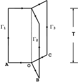
Figure 1: The 3Q Wilson loop $W_{\rm 3Q}$. The 3Q state is generated at $t=0$ and is annihilated at $t=T$. The three quarks are spatially fixed in ${\bf R}^{3}$ for $0<t<T$.

Figure 2: The ground-state overlap $C_{0}$ for the 3Q system with smeared link-variables (upper data) and with unsmeared link-variables (lower data). The horizontal axis denotes $L_{\rm min}$. For each 3Q configuration, $C_{0}$ is largely enhanced as $0.8<C_{0}<1$ by the smearing.

3 Theoretical Consideration for the 3Q Ground-State Potential

In this section, we consider the potential form of $V_{\rm 3Q}$ based on QCD. In the short-distance limit, the perturbative QCD is applicable and the Coulomb-type potential appears as the one-gluon-exchange (OGE) result. In the long-distance limit at the quenched level, the flux-tube picture would be applicable from the argument of the strong-coupling QCD [2, 3, 8], and hence a linear-type confinement potential is expected to appear. Actually, the Q-$\bar{\rm Q}$ potential $V_{\rm Q\bar{Q}}$ is well reproduced by the Coulomb-plus-linear potential in the lattice QCD. Then, we conjecture that the 3Q ground-state potential $V_{\rm 3Q}$ is also expressed by a sum of the short-distance OGE result and the long-distance flux-tube result as

$$V_{\rm 3Q}=-A_{\rm 3Q}\sum_{i<j}\frac{1}{|{\bf r}_{i}-{\bf r}_{j}|}+\sigma_{\rm 3Q}L_{\rm min}+C_{\rm 3Q},\quad V_{\rm Q\bar{Q}}(r)=-\frac{A_{\rm Q\bar{Q}}}{r}+\sigma_{\rm Q\bar{Q}}r+C_{\rm Q\bar{Q}},$$ (5)

where $L_{\rm min}$ denotes the minimal length of the total flux tubes linking the three quarks.

Next, we consider the diquark limit, where the 3Q system becomes equivalent to a Q-$\bar{\rm Q}$ system, which leads to a physical requirement on the relation between $V_{\rm 3Q}$ and $V_{\rm Q\bar{Q}}$. Here, the constant term is to be considered carefully, because there appears a divergence from the Coulomb term in $V_{\rm 3Q}$ as $\frac{-A_{\rm 3Q}}{|{\bf r}_{i}-{\bf r}_{j}|}\rightarrow-\infty$ in the continuum diquark limit. In the lattice regularization, this ultraviolet divergence is regularized to be a finite constant with the lattice spacing $a$ as $\frac{-A_{\rm 3Q}}{|{\bf r}_{i}-{\bf r}_{j}|}\rightarrow\frac{-A_{\rm 3Q}}{\omega a}$, where $\omega$ is a dimensionless constant satisfying $0<\omega<1$ and $\omega\sim 1$. Thus, we get the diquark-limit requirement on the lattice,

$$\sigma_{\rm 3Q}=\sigma_{\rm Q\bar{Q}},\qquad A_{\rm 3Q}=\frac{1}{2}A_{\rm Q\bar{Q}},\qquad C_{\rm 3Q}-C_{\rm Q\bar{Q}}=\frac{A_{\rm 3Q}}{\omega a}\quad(>0).$$ (6)

4 Lattice QCD Results for the 3Q Ground-State Potential

We measure the 3Q ground-state potential $V_{\rm 3Q}$ from 210 gauge configurations in the SU(3)_c lattice QCD using the smearing technique, and compare the lattice data with the theoretical form of Eq.(5). Table 1 shows the best fit coefficients in $V_{\rm 3Q}$ and $V_{\rm Q\bar{Q}}$ in Eq.(5). Table 2 shows the comparison between the lattice QCD data $V_{\rm 3Q}^{\rm latt}$ and the fitting function $V_{\rm 3Q}^{\rm fit}$ in Eq.(5) with the three coefficients listed in Table 1.

As shown in Table 2, the three-quark ground-state potential $V_{\rm 3Q}$ is well described by Eq.(5) with accuracy better than a few %. From Table 1, we find a universal feature of the string tension, $\sigma_{\rm 3Q}\simeq\sigma_{\rm Q\bar{Q}}$, as well as the OGE result for the Coulomb coefficient, $A_{\rm 3Q}\simeq\frac{1}{2}A_{\rm Q\bar{Q}}$. All the diquark-limit requirements in Eq.(6) are satisfied for $\omega\simeq 0.46$.

Another fitting with the $\Delta$-type flux-tube ansatz [4, 5] seems rather worse, because of unacceptably large $\chi^{2}/N_{\rm DS}\geq 10.9$. However, as an approximation, $V_{\rm 3Q}$ seems described by a simple sum of an effective two-body Q-Q potential with a reduced string tension as $\sigma_{\rm QQ}\simeq 0.53\sigma$. This reduction factor can be naturally understood as a geometrical factor rather than the color factor, since the ratio between $L_{\rm min}$ and the perimeter length $L_{P}$ satisfies $\frac{1}{2}\leq\frac{L_{\rm min}}{L_{P}}\leq\frac{1}{\sqrt{3}}$, which leads to $L_{\rm min}\sigma=L_{P}\sigma_{\rm QQ}$ with $\sigma_{\rm QQ}=(0.5\sim 0.58)\sigma$.

Table 1: The string tension, the Coulomb coefficient and the constant term for the 3Q ground-state potential $V_{\rm 3Q}$ and the Q-$\bar{\rm Q}$ potential $V_{\rm Q\bar{Q}}$ in the lattice unit with $a\simeq$ 0.19fm.

	$\sigma$	$A$	$C$
${\rm 3Q}$	$0.1528(27)$	$0.1316(62)$	$0.9140(201)$
${\rm Q\bar{Q}}$	$0.1629(47)$	$0.2793(116)$	$0.6293(161)$

Table 2: The lattice QCD result for the 3Q ground-state potential $V_{\rm 3Q}^{\rm latt}$ and the fitting function $V_{\rm 3Q}^{\rm fit}$ in Eq.(5) for the 3Q system where the three quarks are put on $(i,0,0)$, $(0,j,0)$ and $(0,0,k)$ in ${\bf R}^{3}$ in the lattice unit. The error of $V_{\rm 3Q}^{\rm latt}$ denotes the statistical error estimated with the jackknife method. (The systematic error is not included.)

$(i,j,k)$	$V_{\rm 3Q}^{\rm latt}$	$V_{\rm 3Q}^{\rm fit}$	$V_{\rm 3Q}^{\rm latt}-V_{\rm 3Q}^{\rm fit}$
$(0,1,1)$	0.8459(36)	0.8529	0.0070
$(0,1,2)$	1.0970(40)	1.1023	0.0053
$(0,1,3)$	1.2935(39)	1.2926	$-$0.0009
$(0,2,2)$	1.3164(40)	1.3262	0.0098
$(0,2,3)$	1.5032(58)	1.5069	0.0037
$(0,3,3)$	1.6741(40)	1.6808	0.0067
$(1,1,1)$	1.0231(38)	1.0091	$-$0.0140
$(1,1,2)$	1.2181(61)	1.2145	$-$0.0036
$(1,1,3)$	1.4154(49)	1.3958	$-$0.0196
$(1,2,2)$	1.3870(46)	1.3887	0.0017
$(1,2,3)$	1.5588(60)	1.5580	$-$0.0008
$(1,3,3)$	1.7141(43)	1.7195	0.0054
$(2,2,2)$	1.5216(33)	1.5230	0.0014
$(2,2,3)$	1.6745(11)	1.6755	0.0010
$(2,3,3)$	1.8242(54)	1.8169	$-$0.0073
$(3,3,3)$	1.9607(92)	1.9438	$-$0.0169

References

- [1] T.T. Takahashi, H. Matsufuru, Y. Nemoto and H. Suganuma, Proc. of the TMU-Yale Symp. on “Dynamics of Gauge Fields”, TMU, Tokyo, Dec. 1999, A. Chodos et al. (eds.), Universal Academy Press, Tokyo (2000) in press.
- [2] S. Capstick and N. Isgur, Phys. Rev. D34 (1986) 2809.
- [3] N. Brambilla, G.M. Prosperi and A. Vairo, Phys. Lett. B362 (1995) 113.
- [4] R. Sommer and J. Wosiek, Phys.Lett.149B (1984) 497; Nucl.Phys.B267 (1986) 531.
- [5] H.B. Thacker, E. Eichten and J.C. Sexton, Nucl. Phys. B (Proc. Suppl.) 4 (1988) 234.
- [6] APE Collaboration, M. Albanese et al., Phys. Lett. B192 (1987) 163.
- [7] G.S. Bali, C. Schlichter and K. Schilling, Phys. Rev. D51 (1995) 5165.
- [8] J. Kogut and L. Susskind, Phys. Rev. D11 (1975) 395.