The Phase Diagram of Four Flavor SU(2) Lattice Gauge Theory at Nonzero Chemical Potential and Temperature

Abstract

$SU(2)$ lattice gauge theory with four flavors of quarks is simulated at nonzero chemical potential $\mu$ and temperature $T$ and the results are compared to the predictions of Effective Lagrangians. Simulations on $16^{4}$ lattices indicate that at zero $T$ the theory experiences a second order phase transition to a diquark condensate state. Several methods of analysis, including equation of state fits suggested by Chiral Perturbation Theory, suggest that mean-field scaling describes this critical point. Nonzero $T$ and $\mu$ are studied on $12^{3}\times 6$ lattices. For low $T$, increasing $\mu$ takes the system through a line of second order phase transitions to a diquark condensed phase. Increasing $T$ at high $\mu$, the system passes through a line of first order transitions from the diquark phase to the quark-gluon plasma phase. Metastability is found in the vicinity of the first order line. There is a tricritical point along this line of transitions whose position is consistent with theoretical predictions.

I Introduction

Recently there has been a resurgence of interest in QCD at nonzero chemical potential for quark number. Arguments based on instantons [1] and phenomenological gap equations [2] support the old idea that diquark condensation and a color superconductivity phase transition [3, 4] will occur at a critical chemical potential somewhat greater than that at which nuclear matter forms. Nuclear matter is expected to be the ground state of QCD above a chemical potential $\mu_{N}$, which is slightly less than one-third of the proton’s mass. These arguments neglect the forces of confinement and may only be reliable at asymptotically large chemical potentials. Since diquarks carry color in real QCD, a quantitative understanding of confinement and screening is needed to estimate the energies of the states which control the phases of the system. Unfortunately, brute force lattice simulation methods, which are so useful at $T\neq 0$ and $\mu=0$, do not yet provide a reliable simulation algorithm for these environments in which the fermion determinant becomes complex.

Given these problems, theorists have turned to simpler models which can be analyzed and simulated by current methods. One of the more interesting is the color $SU(2)$ version of QCD which addresses some of the issues of interest [1], [2], [5]. In this model diquarks do not carry color, so their condensation does not break color symmetry dynamically. Instead, the diquark condensed phase resembles a superfluid rather than a superconductor. The critical chemical potential is also expected to be one-half the mass of the lightest meson, the pion, because quarks and anti-quarks reside in equivalent representations of the $SU(2)$ color group. Hence hadron flavor multiplets include both mesons and diquarks. Chiral Lagrangians can be used to study the diquark condensation transition in this model because the critical chemical potential vanishes in the chiral limit, and the model has a Goldstone realization of the spontaneously broken quark-number symmetry [6, 7, 8, 9]. The problem has also been studied within a Random Matrix Model at non-zero $\mu$ and $T$ [10]. Lattice simulations of the model are also possible because the fermion determinant is real and non-negative for all chemical potentials. One hopes that these developments will uncover generic phenomena that will also apply to QCD at nonzero chemical potential. Furthermore, most of the theories that aim at a description of the phase diagram of 3-color QCD at nonzero baryon chemical potential and temperature can be implemented to describe the phase diagram of 2-color QCD at nonzero baryon chemical potential and temperature. Therefore, an important motivation to conduct Lattice simulations is to check the validity of these theories in the 2-color case. If a theory is not correct in the two-color case, it is very doubtful that the predictions of the corresponding 3-color theory can be trusted.

Preliminary lattice simulations of the $SU(2)$ model with four species of quarks, simulation data and an Effective Lagrangian analysis of aspects of the $T$-$\mu$ phase diagram were recently published [11, 12]. It is the purpose of this article to present the continuation of that work on larger lattices, closer to the theory’s continuum limit with a focus on the system’s phase diagram at nonzero $\mu$ and $T$. Very early work on this model at finite $T$ and $\mu$ was performed by [13]. A simulation study of the spectroscopy of the light bosonic modes will be presented elsewhere [14].

In our exploratory study [12] of this model’s phase diagram, we found an unanticipated result. At fixed but small quark mass, which insures us that the pion has a nonzero mass and chiral symmetry is explicitly broken, we found that at high $T$ and $\mu$ there is a line of transitions separating a quark-gluon plasma phase from one with a diquark condensate. Along this line there is a tricritical point, labeled $2$ in Fig. 1, where the transition switches from being second order (and well described by mean field theory) at relatively low $\mu$ to a first order transition at an intermediate $\mu$ value. We will present evidence here for metastability along the line of high $\mu$ and $T$. We have argued elsewhere [12] that this simulation result, the existence of a tricritical point $2$, has a natural explanation in the context of chiral Lagrangians. Following the formalism of [6] we argued that trilinear couplings among the low lying boson fields of the Lagrangian become more significant as $\mu$ and $T$ increase and they can cause the transition to become first order at a $\mu$ value in the vicinity of the results found in the simulation. Using hindsight, this behavior should not have come as a surprise. $\mu$ plays the rôle of a second ‘temperature’ in this theory in that it is a parameter that controls diquark condensation, but does not explicitly break the (quark-number) symmetry. The existence of two competing ‘temperatures’ is a characteristic of systems which exhibit tricritical behavior. A tricritical point is also found in Chiral Perturbation Theory, as well as in a new Random Matrix Theory model [15, 16].

FIG. 1.: Schematic Phase Diagram in the $T$-$\mu$ Plane. The thin(thick) line consists of second(first) order transitions. The dashed line denotes a crossover. Point 1 labels a critical point and Point 2 labels a tricritical point. The existence and position of point 1 is a matter of conjecture in the two color model.

The conjectured phase diagram of Fig. 1 also has a critical point labeled $1$ which connects the line of first order transitions to the dashed line of crossover phenomena extending to the $\mu=0$ axis where we expect a finite T chiral transition between conventional hadronic matter and the quark-gluon plasma. For sufficiently light quarks in the four flavor SU(2) model, the $\mu=0$ transition is known to be first order both from theoretical arguments [17, 18] and simulations [19]. For quark mass $m=0.05$ we find that the transition is smoothed out to a crossover region as $\mu$ is increased until the dynamics favors diquark condensation. Clearly, the results will depend on the precise value of the quark mass $m$. At $m=0.05$ we find that the transition at $\mu=0.10$ is as smooth as that at $\mu=0.0$, while the transition at $\mu=0.20$ is noticeably sharper. This result suggests that if $m$ were chosen somewhat smaller than $m=0.05$, the scenario with the critical point 1 and the first order line might emerge. However, this critical point 1 might be absent so the crossover line would intersect the curve separating the diquark condensation phase from the normal phase. We will be pursuing this suggestion in separate simulations. The simulations done here are not accurate enough to probe the details of the region of the phase diagram Fig. 1 where the two first order lines split apart. Simulations at lower quark masses on larger lattices might be needed.

In QCD at nonzero baryon chemical potential Fodor and Katz [20] have estimated the position of the critical point 1 using a modified, multivariable Glasgow algorithm [21]. It will be interesting to find point 1 in the four flavor SU(2) model at smaller $m$ values using our conventional simulation methods and then checking whether the Fodor-Katz method can find it with competitive accuracy. If point 1 is absent, the Fodor-Katz method should be able to find the intersection of the crossover line with the curve delimiting the diquark phase.

We also present extensive and accurate simulation results on a $16^{4}$ lattice, essentially at vanishing $T$. The critical indices of the transition at nonzero $\mu$ are measured and favor mean-field scaling in agreement with Chiral Perturbation Theory, analyzed through one loop corrections, and simulations of 2-color QCD in the strong coupling limit [22]. The critical indices $\beta_{mag}$ and $\delta$ are emphasized. Equation of State fits, suggested by Chiral Perturbation Theory, also support these conclusions. As a third method to determine the critical indices, we use the static scaling hypothesis. This analysis is also compatible with mean field, although this approach is unable to predict the index $\delta$ accurately because of its sensitivity to estimates of the critical chemical potential, $\mu_{c}$. Unfortunately, because simulations at small $\lambda$ are extremely costly in computing requirements, we have not been able to approach the critical point closely enough to make definitive measurements, insensitive to the detailed nature of the critical scaling. In a recent paper in which we study quenched versions of this and closely related theories, we have indicated how sensitive measurements of critical scaling are to the form of the scaling variable [23]. This paper does indicate, however, that there are classes of scaling variables for which there exist extended regions outside of the true scaling window, where the order parameter scales with the correct critical exponents.

II Simulation Method and The Algorithm

The lattice action of the staggered fermion version of this theory is:

$$S_{f}=\sum_{sites}\left\{\bar{\chi}[D\!\!\!\!/\,(\mu)+m]\chi+\frac{1}{2}\lambda[\chi^{T}\tau_{2}\chi+\bar{\chi}\tau_{2}\bar{\chi}^{T}]\right\}$$ (1)

where the chemical potential $\mu$ is introduced by multiplying links in the $+t$ direction by $e^{\mu}$ and those in the $-t$ direction by $e^{-\mu}$ [24]. The diquark source term (Majorana mass term) is added to allow us to observe spontaneous breakdown of quark-number on a finite lattice. The parameter $\lambda$ and the usual mass term $m$ control the amount of explicit symmetry breaking in the lattice action. We will be particularly interested in small values of $\lambda$ and the extrapolation $\lambda\rightarrow 0$ for a given $m$ to produce an interesting, realistic physical situation. This is the system that has been studied analytically using effective Lagrangians at non-zero chemical potential $\mu$ [6, 7], and non-zero temperature [15].

Integrating out the fermion fields in Eq.1 gives:

$$pfaffian\left[\begin{array}[]{cc}\lambda\tau_{2}&{\cal A}\\ -{\cal A}^{T}&\lambda\tau_{2}\end{array}\right]=\sqrt{{\rm det}({\cal A}^{\dagger}{\cal A}+\lambda^{2})}$$ (2)

where

$${\cal A}\equiv D\!\!\!\!/\,(\mu)+m$$ (3)

Note that the pfaffian is strictly positive, so that we can use the hybrid molecular dynamics [25] method to simulate this theory using “noisy” fermions to take the square root, giving $N_{f}=4$.

For $\lambda=0$, $m\neq 0$, $\mu\neq 0$ we expect no spontaneous symmetry breaking for small $\mu$. For $\mu$ large enough ($\mu>m_{\pi}/2$ according to most approaches including Chiral Perturbation Theory [6, 7, 8]) we expect spontaneous breakdown of quark number and one Goldstone boson – a scalar diquark. (The reader should consult [5] for a full discussion of the symmetries of the lattice action, remarks about spectroscopy, Goldstone as well as pseudo-Goldstone bosons, and for early simulations of the 8 flavor theory at $\lambda=0$.)

III Simulation Results and Analysis

We now consider the simulation results for the $N_{f}=4$ theory on $16^{4}$, $8^{4}$ and $12^{3}\times 6$ lattices, measuring the chiral ($\langle\bar{\chi}\chi\rangle$) and diquark condensates ($\langle\chi^{T}\tau_{2}\chi\rangle$), the fermion number density, the Wilson/Polyakov line, etc.

FIG. 2.: $\langle\chi^{T}\tau_{2}\chi\rangle$ as a function of $\mu$ on an $8^{4}$ lattice at $\beta=1.5$, $m=0.025$. The unlabeled squares are a linear extrapolation to $\lambda=0$

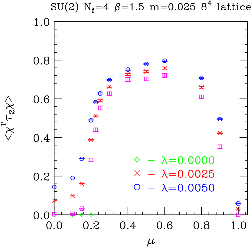
Let us first briefly mention our $8^{4}$ simulations. These were performed at $\beta=1.5$, a relatively strong coupling, and $m=0.025$. These extend our earlier work with the same $\beta$ but $m=0.1$. Using a smaller quark mass increases the validity of chiral perturbation analyses. In addition, we are performing simulations on a $12^{3}\times 24$ lattice with the same parameters to examine the spectrum of Goldstone and pseudo-Goldstone bosons of this theory. For this purpose it is necessary to have the pion mass significantly lighter than that of non-Goldstone, non-pseudo-Goldstone excitations. We have simulated at $\lambda=0.0025$, and $0.005$. Our measurements of the diquark condensate are given in figure 2. Each ‘data’ point represents a 2000 molecular-dynamics time-unit simulation. The fact that a simple linear extrapolation of our measurements to $\lambda=0$ is very small, not only at $\mu=0$, where we know that the condensate vanishes, but also at $\mu=0.1$ leads us to believe that the condensate vanishes in this limit, probably up to $\mu\sim 0.2$. (Note that is is known that there is some small but finite value of $\mu$, below which this condensate vanishes [22].) For $\mu$ much greater than $0.2$ but less than the saturation value it is reasonably clear that the condensate does not vanish in the limit as $\lambda\rightarrow 0$ (on an infinite lattice). Hence there is a phase transition for some value of $\mu$ to a state where quark number is spontaneously broken by a diquark condensate. The transition occurs over a relatively small range of $\mu$, but does not appear to be first order. Because of the relatively small scaling window this implies, we will not be able to analyze critical scaling until we perform measurements at more $\mu$ values within this scaling window.

The chiral condensate remains approximately constant up to $\mu=\mu_{c}$ after which it falls rapidly approaching zero for large $\mu$. The fermion density rises slowly and approximately linearly from zero for $\mu\geq\mu_{c}$. Above $\mu\approx 0.6$, it increases more rapidly approaching its saturation value of $2$ at $\mu\approx 1.0$.

We now turn to measurements on a $16^{4}$, ‘zero temperature’ lattice. We simulated the $SU(2)$ model at a relatively weak coupling $\beta=1.85$, within the theory’s apparent scaling window, in order to attempt to make contact with the theory’s continuum limit. The quark mass was $m=0.05$, as in [12], and a series of simulations were performed at $\lambda=0.0025$, $0.005$, and $0.01$ so that our results could be extrapolated to vanishing diquark source, $\lambda=0$. Simple linear and spline extrapolations were used and these procedures appeared to be sensible away from the transition. None of the conclusions to be drawn here will depend strongly on the limit. In fact, everything we say could be gathered from our data at a fixed (small) $\lambda$ value, $0.005$ or $0.0025$, say. However, only in the limit of vanishing $\lambda$ do we expect real diquark phase transitions (at least when the transitions are second order), so it is particularly interesting and relevant to investigate the $\lambda\rightarrow 0$ limit. The quantitative agreement between fits at fixed, small $\lambda$ values and those using extrapolated data enforce the prevalent idea that simple extrapolation procedures are reliable except in the immediate vicinity of the critical point where non-analyticities are inevitable.

Because we are forced by practical considerations to work at $\lambda$ values large enough that the condensate is relatively smooth over the transition region, we have to deduce critical scaling from the curvature of the condensate further from $\mu_{c}$ than we would like. Thus we run the risk that we are outside the scaling window and the apparent scaling we are seeing does not represent true critical scaling. However, we saw for quenched theories [23] at relatively weak couplings, that the form of the natural scaling variable is such that it has an inflection point when expressed in terms of the simplest scaling variable $\mu-\mu_{c}$. This leads to an extended domain where the order parameter scales with the true critical exponents. It is reasonable to assume that dynamical theories behave similarly.

In Table I we present the raw data on the $16^{4}$ lattice at the three $\lambda$ values. Table II exhibits the results of extrapolating this data to $\lambda=0$. Typically, one thousand time units of the Hybrid Molecular Dynamics algorithm were accumulated to generate these data sets. The error bars in the data sets of Table I account for the correlations in the raw data sets. The low $\lambda$ runs were our most CPU intensive.

Since the Hybrid algorithm suffers from systematic errors proportional to the square of the discrete time step used in integrating its stochastic differential equations forward in Monte Carlo time [25], we were forced to a small discrete time step. The simulations reported here used time steps as small as $dt=0.0025$ to control these errors. Even then, because our statistical errors are so small, these systematic errors might not be negligible. We will later indicate cases where we used $dt$ values which were larger than optimal and have seen signs of such errors.

Now let us discuss some results. In Fig. 3 we show the diquark condensate linearly extrapolated to $\lambda=0$ plotted against the chemical potential $\mu$. The quark mass $m$ was fixed at $0.05$, the coupling was $\beta=1.85$ and the linear extrapolation used the raw data at $\lambda=0.0025$ and $0.005$.

FIG. 3.: Diquark Condensate vs. $\mu$

We see evidence to a quark-number violating second order phase transition in this figure. The dashed line is a power law fit from $\mu=0.30$ to $0.35$ which predicts the critical chemical potential of $\mu_{c}=0.2860(2)$. The power law fit is good, its confidence level is $48$ percent, and its critical index is $\beta_{mag}=0.54(3)$ which is consistent with the mean field result $\beta_{mag}=1/2$, predicted by chiral perturbation theory [6], [7] including one loop corrections. Note that the quark mass is fixed at $m=0.05$ throughout this simulation, so chiral symmetry is explicitly broken and the transition of Fig. 2 is due to quark number breaking alone.

In figure 4 we show the diquark data extrapolated to $\lambda=0$ quadratically using the raw data at $\lambda=0.010$, $0.005$ and $0.0025$. The fit to the data at $\mu$ ranging from $0.30$ through $0.35$ is also shown. The fit predicts a critical point $\mu_{c}=0.2870(2)$, has a confidence level of $47$ percent and has a critical exponent of $\beta_{mag}=0.54(4)$, again in agreement with mean field theory.

FIG. 4.: Diquark Condensate vs. $\mu$

Further evidence for $\beta_{mag}=1/2$ can be obtained directly from the raw data without any extrapolations. For example, in figure 5 we show the $\lambda=0.0025$ data and a power law fit ranging form $\mu=0.30$ through $0.38$. We find $\mu_{c}=0.2749(2)$, $\beta_{mag}=0.54(5)$ with a confidence level of $24$ percent.

FIG. 5.: Diquark Condensate vs. $\mu$.

We also considered extrapolations of the form $\langle\chi^{T}\tau_{2}\chi\rangle=\rho$ where $\rho$ is the solution of an equation of the form $\rho^{3}=a\>\rho+b\>\lambda$ with $a$ and $b$ determined as functions of $\mu$ by performing an independent fit at each $\mu$. This form is suggested my mean-field scaling forms, which would predict that $a$ should be proportional to $\mu-\mu_{c}$ close to the transition. However, these fits were so poor that this approach was abandoned.

In addition, we considered the fermion number density which is predicted to rise linearly from $\mu_{c}$ and found good agreement with this expectation, as shown in figure 6.

FIG. 6.: Fermion Number Density vs. $\mu$.

The fit predicts the critical point $\mu_{c}=0.2765(5)$, with a critical index $1.17(7)$ and a confidence level of $13.1$ percent. Plots and fits of the fermion number density at the other $\lambda$ values were equally good. In fact the fermion number density shows relatively little $\lambda$ dependence. This is in agreement with Chiral Perturbation Theory [7].

Finally, we considered the $\lambda=0.005$ simulations and extended the measurements up to large $\mu\rightarrow 1.2$, shown in figure 7. We see the curious phenomenon observed in the past: as $\mu$ becomes large, the condensate falls to zero. The point is that once $\mu$ becomes of order unity, the discreteness of the lattice comes into play and suppresses the density of states which forces the condensate to fall toward zero. The quark-number density approaches 2 (per lattice site), the maximum allowed by Fermi statistics. This is a lattice artifact. Nonetheless, we can try a power law fit to the diquark condensate over the entire region of $\mu$ from $0.30$ to $0.60$ where the curve is increasing. The result is shown in the figure and the fit predicts $\beta_{mag}=0.49(7)$ and $\mu_{c}=0.2651(2)$. Since $\chi^{2}/dof\sim 5$, the fit is poor, but the deviations from this fit are small enough that this fit should be considered a reasonable zeroth order approximation.

FIG. 7.: Diquark Condensate vs. $\mu$.

In summary, $\beta_{mag}$ measurements are relatively easy and self-consistent. For all the parameters and procedures we tried, we found good agreement with mean field theory. It was important, however, to be working at relatively weak coupling, $\beta=1.85$, in the theory’s scaling window where such an extended scaling window exists. Experience has shown that at stronger coupling, the true scaling is described by effective Lagrangians closer to the non-linear sigma model form, where the scaling window in $\mu-\mu_{c}$ is small and the extended scaling regime exhibits scaling in $\mu-\mu_{c}$ but with an apparent critical exponent $\beta_{m}$ which is half the true value [22, 23, 26].

A second critical index in which we are interested is $\delta$, which controls the response of the system to symmetry breaking fields at the critical point $\mu_{c}$,

$$\langle\chi^{T}\tau_{2}\chi\rangle=A\lambda^{1/\delta}$$ (4)

in the limit of small $\lambda$. Mean field theory predicts $\delta=3$. This scaling law Eq. 4 is usually difficult to use in practice because first it requires accurate estimates of $\mu_{c}$, and second it generally suffers from a small scaling window in $\lambda$. Not having a precise estimate of $\mu_{c}$ is probably our biggest problem, since as we have shown in [23], fits to the extended scaling regime can underestimate $\mu_{c}$ by $\approx 8\%$. In order to obtain some useful data, however, we simulated the $16^{4}$ lattice for four estimates of $\mu_{c}$ each over a range of $\lambda$ from $0.002$ to $0.010$. First we note that the chosen $dt$ for the $\lambda=0.002$ simulations was too large and although plotted on our graphs, these points were excluded from our fits.

We considered $0.2855$, $0.2870$, $0.2920$ and $0.2970$ as estimates of $\mu_{c}$ and tried fits of the form $A\lambda^{1/\delta}+B$. The data and fits are shown in the next four figures, which we discuss in turn.

The $\mu=0.2855$ data predicted $\delta=4.0(6)$ with a confidence level of $91$ percent, but with a large, negative constant $B=-0.17(7)$. The fit considers the data from $\lambda$ ranging from $0.004$ to $0.010$ because the data at $\lambda=0.002$ has large $dt^{2}$ errors. These results are shown in figure 8 The fact that $B$ is large and negative suggests that this estimate for $\mu_{c}$ is too low.

In figure 9 we consider the same ideas for the estimate $\mu_{c}=0.2870$ and now find $\delta=2.5(2)$ and $B=-0.02(2)$, but with a rather poor confidence level of a few percent. For $\mu_{c}=0.2920$ (figure 10), we find $\delta=2.1(2)$, but $B$ is distinctly different from zero, $B=0.05(2)$. The confidence level is, however, very good, $96$ percent. Finally, for $\mu_{c}=0.2970$ we find $\delta=2.7(6)$ and $B=0.02(4)$ with a confidence level of about one percent. See figure 11.

FIG. 8.: Diquark Condensate vs. $\lambda$ for $\mu_{c}=0.2855$

FIG. 9.: Diquark Condensate vs. $\lambda$ for $\mu_{c}=0.2870$

FIG. 10.: Diquark Condensate vs. $\lambda$ for $\mu_{c}=0.2920$

FIG. 11.: Diquark Condensate vs. $\lambda$ for $\mu_{c}=0.2970$

In summary, $\delta$ is in the mean field ‘ballpark’, but the uncertainly in the simulation results is large. The results give us no reason to doubt the application of mean field theory because they are all in the vicinity of $\delta=3$ with some fits higher and some lower. The sensitivity of the simulation estimates to $\mu_{c}$ is considerable. We learn from these measurements that only a focused set of measurements that determine $\mu_{c}$ very well will produce a useful estimate of $\delta$.

IV Comparison with Chiral Perturbation Theory

It is interesting to compare the lattice data to the theoretical predictions of Chiral Perturbation Theory. Two-color QCD at non-zero baryon/quark-number chemical potential has been thoroughly studied at the tree level and at next-to-leading order within Chiral Perturbation Theory [6, 7, 8]. At next-to-leading order, it was found that the phase transition between the normal phase and the superfluid diquark phase is second order, that the critical chemical potential is given by $\mu_{c}=m_{\pi}/2$ and that the critical exponents are given by mean-field theory. Furthermore, based on the structure of the loop corrections, it was conjectured that the critical exponents are given by mean field at any (finite) order in Chiral Perturbation Theory [8].

Overall, the next-to-leading-order corrections do not dramatically change the leading-order results [8]. The corrections turn out to be small, as long as $\mu$ is close to $\mu_{c}$. Therefore it should be enough to compare the lattice data to Chiral Perturbation Theory at leading-order, at least for the lattices sizes, couplings and parameters considered here.

In Chiral Perturbation Theory at leading order, the diquark condensate at non-zero diquark source is given by

$$\langle\chi^{T}\tau_{2}\chi\rangle=\langle\bar{\chi}\chi\rangle_{0}\sin\alpha,$$ (5)

where $\langle\bar{\chi}\chi\rangle_{0}$ is the chiral condensate at zero chemical potential, zero temperature, and zero diquark source, and $\alpha$ is given implicitly by

$$4\mu^{2}\cos\alpha\sin\alpha=m_{\pi}^{2}\sin(\alpha-\phi).$$ (6)

In the equation above $\tan\phi=\lambda/m$, and $m_{\pi}$ is the mass of the Goldstone modes at chemical potential $\mu=0$, temperature $T=0$, and diquark source $\lambda=0$ [7]. Furthermore the quark-antiquark (chiral) condensate is given by

$$\langle\bar{\chi}\chi\rangle=\langle\bar{\chi}\chi\rangle_{0}\cos\alpha.$$ (7)

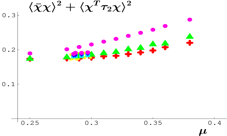
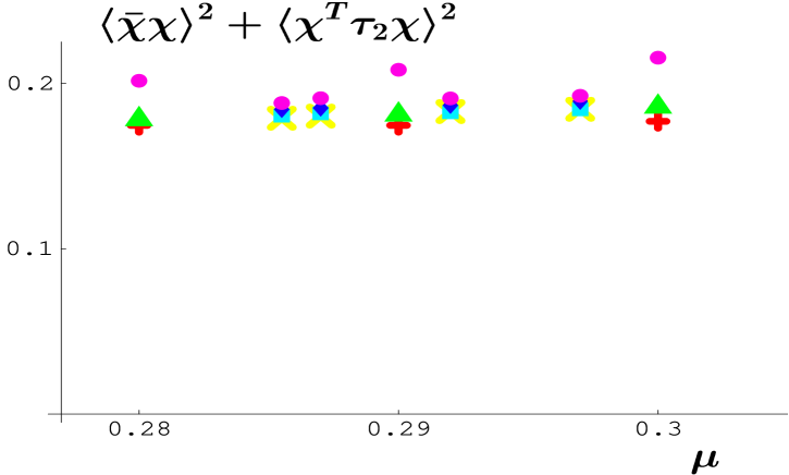
At nonzero diquark source there is a crossover between the normal phase and the diquark condensation phase. However, Chiral Perturbation Theory at leading order predicts that $\langle\bar{\chi}\chi\rangle^{2}+\langle\chi^{T}\tau_{2}\chi\rangle^{2}$ does not depend on the chemical potential, the diquark source, or the quark mass. This relation does not hold at next-to-leading order in Chiral Perturbation Theory [8]. However, for small chemical potential, quark mass and diquark source, Chiral Perturbation Theory at leading order should give an accurate description of these observables. Therefore, we expect that $\langle\bar{\chi}\chi\rangle^{2}+\langle\chi^{T}\tau_{2}\chi\rangle^{2}$ depends slightly on the quark mass and the diquark source, in the same way as the quark-antiquark condensate depends on the quark mass in three-color QCD at zero temperature and chemical potential [27]. The behavior of $\langle\bar{\chi}\chi\rangle^{2}+\langle\chi^{T}\tau_{2}\chi\rangle^{2}$ is presented in Figure 12. These graphs confirm what was expected from Chiral Perturbation Theory: $\langle\bar{\chi}\chi\rangle^{2}+\langle\chi^{T}\tau_{2}\chi\rangle^{2}$ is close to constant for small enough $\mu$ and $\lambda$. Notice that it is impossible to see the critical chemical potential, which is around $0.29$ as determined in the previous section, by looking at $\langle\bar{\chi}\chi\rangle^{2}+\langle\chi^{T}\tau_{2}\chi\rangle^{2}$. The points at $\lambda=0.010$ show the effects of finite $dt^{2}$ errors. The points which lie higher were generated in simulations with $dt=0.01$ while the 4 lower points were generated in simulations with $dt=0.005$.

FIG. 12.: $\langle\bar{\chi}\chi\rangle^{2}+\langle\chi^{T}\tau_{2}\chi\rangle^{2}$ for different diquark sources and chemical potentials. The pluses are the lattice data for $\lambda=0.025$, the xs for $\lambda=0.004$, the triangles for $\lambda=0.005$, the squares for $\lambda=0.006$, the diamonds for $\lambda=0.008$, and the dots for $\lambda=0.010$. a) shows that $\langle\bar{\chi}\chi\rangle^{2}+\langle\chi^{T}\tau_{2}\chi\rangle^{2}$ is almost constant for $0.28\leq\mu\leq 0.30$ and for a given diquark source. b) shows the transition region on an expanded scale.

We could compare the diquark condensate obtained on the lattice with the leading-order result (5). But we notice that within Chiral Perturbation Theory at leading order we have that

$$\frac{\langle\chi^{T}\tau_{2}\chi\rangle}{\langle\bar{\chi}\chi\rangle}=\tan\alpha.$$ (8)

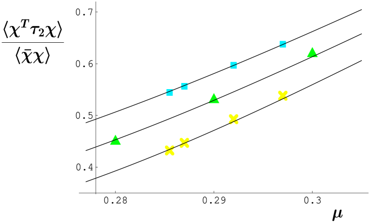
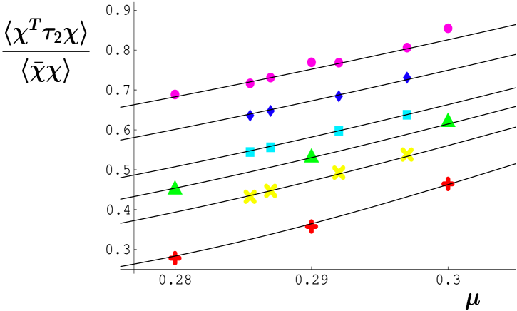
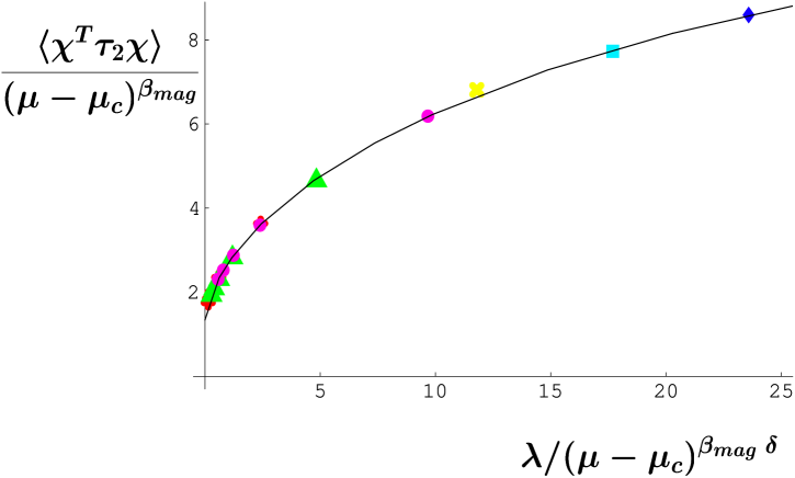
This observable can also be used as an order parameter of the diquark condensation phase. In Chiral Perturbation Theory at leading order, for a given quark mass, diquark source and chemical potential, the ratio (8) only depends on the value of the pion mass $m_{\pi}$ through the minimization equation (6). It is therefore a very suitable observable to use in the comparison between the lattice results and Chiral Perturbation Theory.

Hence we fit the lattice result for $\langle\chi^{T}\tau_{2}\chi\rangle/\langle\bar{\chi}\chi\rangle$ with Chiral Perturbation Theory (8,6). This is a one-parameter fit. Since we use Chiral Perturbation Theory at leading order to analyze our results, we can only take into account data corresponding to chemical potentials and diquark sources that are small enough so that $\langle\bar{\chi}\chi\rangle^{2}+\langle\chi^{T}\tau_{2}\chi\rangle^{2}$ is constant for a given diquark source. The previous figure shows that we have to limit our analysis to data corresponding to $0.28\leq\mu\leq 0.30$, where $\langle\bar{\chi}\chi\rangle^{2}+\langle\chi^{T}\tau_{2}\chi\rangle^{2}$ is close to constant for a given diquark source. If we use the 11 points that correspond to $\lambda=0.004$, $0.005$, and $0.006$, and $0.28\leq\mu\leq 0.30$, we get that $\mu_{c}=0.3027(1)$. This is an acceptable fit since $\chi^{2}/dof=2.3$ (remembering that the norm of the condensate is only approximately constant over this range.) This one-parameter fit and the data we used to perform it are shown in Figure 13a. If we now use the 18 points that correspond to $\lambda=0.0025$, $0.004$, $0.005$, $0.006$, and $0.008$, and $0.28\leq\mu\leq 0.30$, we get that $\mu_{c}=0.3028(1)$, and the fit has a $\chi^{2}/dof=3.1$. If we use the 25 points that correspond to $\lambda=0.0025$, $0.004$, $0.005$, $0.006$, $0.008$, and $0.010$, and $0.28\leq\mu\leq 0.30$, we get that $\mu_{c}=0.3026(2)$. The fit is worse than the previous ones with a $\chi^{2}/dof=12$. This one-parameter fit and the data we used to perform it are shown in Figure 13a. Again we note that the 3 points at $\lambda=0.010$ which lie above the curve are those with $dt=0.01$ which have larger $dt^{2}$ errors, and are largely responsible for this large $\chi^{2}$.

Noting that the new estimates for $\mu_{c}$ are significantly higher than our previous estimates, we consider the inclusion of the ‘data’ at $\mu=0.31$ and $\mu=0.32$ in our fits. If we include the measurements from $\mu=0.31$ to the 25 points that correspond to $\lambda=0.0025$, $0.004$, $0.005$, $0.006$, $0.008$ used in the fits of the previous paragraph, the $\chi^{2}/dof$ increases from $3.1$ to $4.9$. Including both the $\mu=0.31$ and $\mu=0.32$ measurements further increases the $\chi^{2}/dof$ to $5.9$. In both cases the new $\mu_{c}$ is entirely consistent with the estimates of the previous paragraph.

FIG. 13.: Comparison between Chiral Perturbation Theory and the lattice results for $\langle\chi^{T}\tau_{2}\chi\rangle/\langle\bar{\chi}\chi\rangle$. The pluses are the lattice data for $\lambda=0.025$, the xs for $\lambda=0.004$, the triangles for $\lambda=0.005$, the squares for $\lambda=0.006$, the diamonds for $\lambda=0.008$, and the dots are for $\lambda=0.010$. The results of two different fits with Chiral Perturbation Theory and the data we used for these fits are depicted in the solid curves for the different diquark sources: a) for $\lambda=0.004,0.005,0.006$ only; b) for all $\lambda$s.

In summary, we find that Chiral Perturbation Theory at leading order describes the data well, with a critical chemical potential given by $\mu_{c}=0.3027(3)$. This is somewhat higher than our earlier estimates in the previous section, and might explain why our $\delta$ estimates were less than compelling. It is also understandable in terms of what was learned from the quenched studies performed in [23]. In Chiral Perturbation Theory, the critical exponents are given by mean-field theory even at next-to-leading order. From the quality of the fits of the lattice results with Chiral Perturbation Theory that are presented above, we conclude that the critical exponents measured on the lattice are consistent with mean field.

We notice that Chiral Perturbation Theory at leading order does not describe the data very well at large chemical potential and diquark source. This is presumably a sign that higher order corrections have to be taken into account. The introduction of $\mu$ breaks the original symmetry and allows the condensates to vary independently. This can, in part, be implemented by replacing the effective potential based on non-linear sigma models, by a phenomenological effective potential suggested by linear sigma models, where the condensates are less tightly constrained [23].

V Scaling function

The static scaling hypothesis states that the data for $\langle\chi^{T}\tau_{2}\chi\rangle/(\mu-\mu_{c})^{\beta_{mag}}$ for different diquark sources and chemical potentials should collapse onto a single curve for $\mu>\mu_{c}$ when plotted against $\lambda/(\mu-\mu_{c})^{\Delta}$ [28]. The gap exponent $\Delta=\beta_{mag}\delta$; $\Delta=3/2$ in mean-field theory. We can fit the lattice results to the scaling function if we assume some form for the scaling function. We will try several possibilities for the form of the scaling function: linear, of the form $f(x)=a+bx^{s}$, of the form $f(x)=a+bx+cx^{2/3}$ and the simplest mean-field form. The number of parameters changes according to the assumption for the form of the scaling function. We present our results in Table 4 using part of the data ($\mu=0.297$, $0.30$, $0.31$, $0.32$, $0.33$, and $0.34$).

The different forms assumed for the scaling function give similar results for the critical chemical potential and for the two critical exponents that we studied. The best fit corresponds to a critical chemical potential that is consistent with the result we found in the previous section, $\mu_{c}=0.2948(7)$, a value of $\beta_{mag}=0.58(4)$ which is consistent with mean field, and a value of $\delta=2.28(3)$ which is about three quarters of the mean-field result. None of these fits are very good: the best fit has a $\chi^{2}/dof=17$. It corresponds to the scaling function of the form $f(x)=a+bx+cx^{2/3}$, as presented in Table VI. In Figure 14, we show the scaling function together with the $95\%$-confidence ellipse for the parameters $\beta_{mag}$ and $\delta$ using the best fit.

FIG. 14.: Scaling function and $95\%$-confidence ellipse for the critical exponents $\beta_{mag}$ and $\delta$ from our best fit, which corresponds to $\mu_{c}=0.2948$, $\beta_{mag}=0.58$, and $\delta=2.28$. The pluses are the lattice data for $\lambda=0.025$, the xs for $\lambda=0.004$, the triangles for $\lambda=0.005$, the squares for $\lambda=0.006$, the diamonds for $\lambda=0.008$, and the dots for $\lambda=0.010$.

The quality of these fits is rather poor. Furthermore, we find that there is a sizeable correlation between the different fit parameters: $\mu_{c}$ is strongly anti-correlated with $\beta_{mag}$ and mildly with $\delta$, whereas $\beta_{mag}$ and $\delta$ are mildly correlated with each other. Therefore, the results from the fits using the scaling function are somewhat suspect. This can be readily seen by using the same data as above plus the four points that correspond to $\mu=0.2920$. The best fit we get has a $\chi^{2}/dof=66$. It gives $\mu_{c}=0.269(8)$, $\beta_{mag}=0.7(1)$, and $\delta=1.4(2)$. Notice that $\mu_{c}$ is much lower than before, that the increase in $\beta_{mag}$ is sizeable, and that $\delta$ has changed by almost $40\%$. This result illustrates the problems usually encountered in the use of the scaling function. Since the scaling function is in general different above and below the critical point, the choice of data is crucial, and it is difficult to get a clear result from this type of analysis. The comparison with Chiral Perturbation Theory presented in the previous section does not suffer from these problems.

Finally if we impose mean-field exponents, using the same part of the data as above ($\mu=0.297$, $0.30$, $0.31$, $0.32$, $0.33$, and $0.34$), the best fit we get has poor quality: $\chi^{2}/dof=243$. It gives $\mu_{c}=0.297(8)$, which is compatible with the results obtained in the previous section where we compared the data with Chiral Perturbation Theory. If we try to use scaling functions derived from the mean-field equation of state as in [23], the quality of the fit is marginally better, with a $\chi^{2}/dof=205$, and it gives $\mu_{c}=0.308(2)$.

VI Runs at finite temperature

We now present our $12^{3}\times 6$ simulations to investigate the interior of the phase diagram of Fig. 1 . We are particularly interested in scanning the diagram starting at $\mu=0$ and following phase transitions and lines of crossover phenomena at high $T$ out to large $\mu$. In particular, the low mass four flavor theory should have a first order transition on the $\mu=0$ axis and this transition should penetrate into the phase diagram. In addition, the $T=0$ transition to a diquark condensate at $\mu_{c}$ should penetrate into the phase diagram and separate the normal phase from the phase with a diquark condensate as shown in Fig. 1. It would be interesting to understand if and how these two lines of transitions merge inside the phase diagram. Finally, we know from past simulations and Effective Lagrangian analyses that there is a line of first order transitions at high $\mu$ and high $T$ which separates the diquark condensate phase from the quark-gluon plasma phase [12]. We want to confirm the first order character of the high $\mu$ part of this line and to find the low $\mu$ end of this line where it changes to second order at a tricritical point, labeled 2 in Fig. 1. This point has also been found within Chiral Perturbation at nonzero temperature and chemical potential [15].

We are hopeful that some of these features of the phase diagram will also occur in other models, so it would be useful to confirm them in this relatively simple setting. Perhaps, QCD at nonzero Baryon Number chemical potential has a $T$-$\mu$ phase diagram with some of these features.

We begin by considering the $\mu=0$ axis. Our simulations are at nonzero fermion mass $m=0.05$ and non-zero diquark source $\lambda=0.005$ (equivalent to running at $m=\sqrt{0.05^{2}+0.005^{2}}$ ). $m=0.05$ is large enough that we expect the transition between hadronic matter and the quark-gluon plasma to be weakened and perhaps softened into a crossover. This is, in fact, what we find. (At lower quark mass we would expect to find a first order transition.) In Fig. 15 we show data for the chiral condensate and the Wilson Line and confirm a smooth but rapid crossover in the vicinity of $\beta=1.9$.

FIG. 15.: Wilson Line and Condensates vs. $\beta$ for $\mu=0.00$.

Measurements at $\mu=0.10$ gave similar conclusions: there is a clear but smooth crossover in the vicinity of $\beta=1.9$, as shown in figure 16.

FIG. 16.: Wilson Line and Condensates vs. $\beta$ for $\mu=0.10$.

It is interesting that a plot of the same quantities at $\mu=0.20$ displays a noticeably sharper crossover. Figure 17 suggests that $\mu=0.20$ is near a critical point, such as the point 1 in our generic phase diagram, Fig. 1. At this rather large quark mass $m=0.05$, this appears merely to be a more pronounced crossover but, perhaps, if $m$ were chosen smaller than $0.05$, an actual line of first order transitions would be found for the region corresponding to $\mu>0.20$ in this phase diagram.

FIG. 17.: Wilson Line and Condensates vs. $\beta$ for $\mu=0.20$.

Once we increase $\mu$ to $0.25$, the induced diquark condensate becomes more significant at low $T$, as shown in figure 18.

FIG. 18.: Wilson Line, and Condensates vs. $\beta$.

At $\mu=0.30$ the diquark condensate becomes the most interesting and rapidly varying quantity. The chiral condensate is relatively smooth and changes from $0.493(6)$ at $\beta=1.7$ to $0.217(1)$ at $\beta=1.9$ while the diquark condensate has varied from $0.352(5)$ to $0.0400(3)$ over the same range of coupling. The Wilson Line varies from $0.057(3)$ to $0.241(2)$ over the same range. As shown in the figure 19, the diquark condensate experiences a sharp transition between $\beta=1.80$ and $1.90$.

FIG. 19.: Wilson Line and Condensates vs. $\beta$.

That transition becomes even sharper as we increase $\mu$ to $0.35$ as shown in figure 20.

FIG. 20.: Wilson Line and Condensates vs. $\beta$.

At $\mu=0.40$, the simulations indicate a first order transition near $\beta=1.85(3)$. In figure 21 we show both the diquark condensates and the Wilson Line and see strong suggestions of discontinuities.

FIG. 21.: Wilson Line and Condensates vs. $\beta$.

The really solid evidence for a first order transition comes from the time evolution of the observables at $\beta=1.87$ which show signs of metastability. For example, in the figure 22 we show the time evolution of the diquark condensate and display several tunnelings between a state having a condensate near $0.15$ and another with a condensate near $0.40$.

FIG. 22.: Diquark Condensate vs. Computer Time.

Runs at $\mu=0.50$ and $0.60$ show clear discontinuities in both the diquark condensate and the Wilson Line near $\beta=1.87$. In figure 23 we show the results for $\mu=0.60$.

FIG. 23.: Wilson Line and Condensates vs. $\beta$.

Finally, we scanned the phase diagram at low $T$ and variable $\mu$. We accumulated data at $\beta=1.30$, relatively strong coupling and near vanishing $T$, on the $12^{3}\times 6$ lattice and took measurements over a wide range of $\mu$, from $0.15$ to $0.60$. The results for the diquark condensate are shown in the figure 24 which shows a transition near $\mu=0.25$. The power law fit shown in the figure produces a critical index $\beta_{mag}=0.29(4)$ at a critical chemical potential $\mu_{c}=0.2453(2)$. The quality of the fit, which extends from $\mu=0.26$ to $0.38$, is rather poor, having a confidence level of only a fraction of one percent. As we have seen in quenched simulations and in simulations of QCD at finite chemical potential for isospin such small estimates of the critical index are often an indication that the scaling is best described in terms of the scaling form for the effective Lagrangian in the non-linear sigma-model class. [23, 26, 29].

FIG. 24.: Diquark Condensate vs. $\mu$.

The estimate for the critical chemical potential, $\mu_{c}=0.2453(2)$, meshes well with our measurements at high $T$ above, which indicated that the diquark condensate only started to be numerically significant for $\mu\gtrsim 0.25$.

The continuous phase transition is also seen in the induced fermion-number density shown in the figure 25. The dotted line fit to that data, which extends all the way from $\mu=0.26$ to $0.56$, has a confidence level of $42$ percent, a critical index $0.99(2)$ and an estimate for the critical chemical potential, $\mu_{c}=.2282(2)$. The scaling law obtained here is in good agreement with field theory expectations of unity. Note that such linearity for these relatively strong couplings has a wider range of validity than would be indicated by the scaling window, as is seen in the explicit scaling forms from effective Lagrangians [6, 7]. Since we only have a single $\lambda$ value, we have not attempted a fit to such a form.

FIG. 25.: Fermion-Number Density vs. $\mu$.

VII Conclusion and Outlook

In this article we have presented a study of the phase diagram of 2-color QCD at nonzero baryon/quark-number chemical potential and nonzero temperature. We have found two phases: a “normal” phase where quark number is conserved and a phase with a diquark condensate which spontaneously breaks quark number. At $\mu=0$, for smaller quark masses, there should be a first order finite temperature “deconfinement” transition which divides the hadronic from the quark-gluon plasma phase. Since, even in this case we expect the line of first order transitions emerging from this point to terminate at small $\mu$, beyond which there should be a rapid crossover but no transition, the hadronic and quark-gluon plasma phases are not distinct. This is the phase we call the “normal” phase. The chiral condensate is non-zero everywhere. However, where it is large the system is more hadronic in nature; where it is small, the system is more plasma-like. In the “diquark” phase, the chiral condensate decreases with increasing diquark condensate, approaching zero for large $\mu$ (even before saturation sets in). We have found that the phase transition between the “normal” phase and the diquark phase for small $T$ is second order and compatible with mean field theory. These simulations therefore agree with the predictions of Chiral Perturbation Theory through next-to-leading order [8].

We have also found that the second order phase transition between the “normal” phase and the diquark phase becomes first order when $\mu$ and $T$ are increased. Therefore the $\mu$-$T$ phase diagram contains a tricritical point. It corresponds to a chemical potential near two-thirds of the pion mass, and a temperature only slightly lower than the transition temperature between the hadronic phase and quark-gluon plasma phase at $\mu=0$. The tricritical point is also found in Chiral Perturbation Theory at nonzero temperature and chemical potential [15]. Therefore, this phase diagram is consistent with the one obtained within Chiral Perturbation Theory [15].

Now that the phase diagram of this theory has been mapped out, we can turn to more quantitative properties. In particular, we plan on analyzing the gauge configurations for their topological content. There are interesting predictions [30] based on Effective Lagrangians for the size, density and interactions among the instantons of the model at large $\mu$ which can be investigated by cooling methods which have been very successful at vanishing $\mu$. In addition, we can simulate the phase diagram at low $\mu$ and high T with lighter quarks and search for the critical point 1. The SU(3) analog of this point is thought to be accessible to heavy ion collisions planned for BNL’s RHIC.

Furthermore, the spectroscopy of the model, with an emphasis on Goldstone and pseudo-Goldstone bosons, is also under consideration. Since the theory’s light modes control its critical behavior and thermodynamics, quantitative results on spectroscopy are quite important.

There are also interesting effective Lagrangian predictions for QCD with chemical potentials associated with the light quarks [31, 32, 33]. We are studying QCD with a chemical potential associated with isospin [26, 15]. This model’s phases at nonzero $\mu$ and temperature $T$ are expected to be very similar to those discussed here [31]. Although we cannot attack the $SU(3)$ theory with a large Baryon number chemical potential, these other situations can be studied both analytically and numerically, and interesting new phases of matter have been found there which should be investigated further.

$\mu$	$<\chi^{T}\tau_{2}\chi>$	$<\chi^{T}\tau_{2}\chi>$	$<\chi^{T}\tau_{2}\chi>$
$.25$	$0.0617(2)$	$0.1134(2)$	$0.1962(4)$
$.28$	$0.1120(5)$	$0.1732(4)$	$0.2546(5)$
$.29$	$0.1407(5)$	$0.1993(5)$	$0.2782(4)$
$.30$	$0.1772(9)$	$0.2269(6)$	$0.3016(5)$
$.31$	$0.2120(6)$	$0.2544(6)$	$0.3240(3)$
$.32$	$0.2415(11)$	$0.2783(7)$	$0.3470(6)$
$.33$	$0.2711(7)$	$0.3045(7)$	$0.3687(5)$
$.34$	$0.2951(11)$	$0.3253(9)$	$0.3893(6)$
$.35$	$0.3200(9)$	$0.3499(7)$	$0.4082(7)$
$.36$	$0.3437(12)$	$0.3651(9)$	$0.4287(6)$
$.38$	$0.3815(13)$	$0.4044(9)$	$0.4627(7)$

TABLE I.: Diquark Condensates on a $16^{4}$ lattice at $\lambda=0.0025$, $0.005$, and $0.010$ in the second, third, and fourth column, respectively. The first column lists the $\mu$ values.

$\mu$	$<\chi^{T}\tau_{2}\chi>$	$<\chi^{T}\tau_{2}\chi>$
$.25$	$0.0100(2)$	$0.0031(2)$
$.28$	$0.0508(5)$	$0.0371(5)$
$.29$	$0.0821(5)$	$0.0693(5)$
$.30$	$0.1275(9)$	$0.1193(9)$
$.31$	$0.1710(6)$	$0.1664(6)$
$.32$	$0.2050(11)$	$0.2031(11)$
$.33$	$0.2380(7)$	$0.2376(7)$
$.34$	$0.2650(11)$	$0.2661(11)$
$.35$	$0.2900(9)$	$0.2896(9)$
$.36$	$0.3220(12)$	$0.3292(12)$
$.38$	$0.3590(13)$	$0.3628(12)$

TABLE II.: Diquark Condensates on a $16^{4}$ lattice at $\lambda=0.00$. The first column lists the $\mu$ values, the second records the linear extrapolations of the diquark condensates and the third records the quadratic extrapolations.

$\mu$	$<\bar{\chi}\chi>$	$<\bar{\chi}\chi>$	$<\bar{\chi}\chi>$
$.25$	$0.4123(5)$	$0.4012(5)$	$0.3887(5)$
$.28$	$0.4025(8)$	$0.3850(6)$	$0.3697(6)$
$.29$	$0.3934(7)$	$0.3758(5)$	$0.3616(4)$
$.30$	$0.3816(9)$	$0.3664(7)$	$0.3529(5)$
$.31$	$0.3686(6)$	$0.3541(6)$	$0.3444(5)$
$.32$	$0.3523(11)$	$0.3409(8)$	$0.3335(6)$
$.33$	$0.3381(6)$	$0.3298(8)$	$0.3234(5)$
$.34$	$0.3242(11)$	$0.3157(8)$	$0.3125(6)$
$.35$	$0.3091(10)$	$0.3057(7)$	$0.3026(7)$
$.36$	$0.2987(12)$	$0.2908(9)$	$0.2920(7)$
$.38$	$0.2733(12)$	$0.2722(9)$	$0.2711(7)$

TABLE III.: Quark-antiquark Condensates on a $16^{4}$ lattice at $\lambda=0.0025$, $0.005$, and $0.010$ in the second, third, and fourth column, respectively. The first column records the $\mu$ values.

$\lambda$	$<\chi^{T}\tau_{2}\chi>$	$<\chi^{T}\tau_{2}\chi>$	$<\chi^{T}\tau_{2}\chi>$	$<\chi^{T}\tau_{2}\chi>$
$.002$	$0.1239(6)$	$0.1315(4)$	$0.1678(8)$	$0.2194(14)$
$.004$	$0.1678(4)$	$0.1732(3)$	$0.1890(5)$	$0.2034(7)$
$.006$	$0.2031(4)$	$0.2073(2)$	$0.2190(4)$	$0.2308(5)$
$.008$	$0.2303(4)$	$0.2338(2)$	$0.2440(4)$	$0.2566(4)$
$.010$	$0.2526(3)$	$0.2579(2)$	$0.2662(3)$	$0.2753(4)$

TABLE IV.: Diquark Condensates on a $16^{4}$ lattice at four estimates of the critical $\mu$, $0.2855$, $0.2870$, $0.2920$, and $0.2970$ in the second, third, fourth, and fifth column, respectively. The first column records the $\lambda$ values.

$\lambda$	$<\bar{\chi}\chi>$	$<\bar{\chi}\chi>$	$<\bar{\chi}\chi>$	$<\bar{\chi}\chi>$
$.002$	$0.4244(9)$	$0.4261(6)$	$0.4362(9)$	$0.452(2)$
$.004$	$0.3882(6)$	$0.3875(4)$	$0.3836(5)$	$0.3780(9)$
$.006$	$0.3730(4)$	$0.3726(3)$	$0.3668(4)$	$0.3619(5)$
$.008$	$0.3622(4)$	$0.3611(3)$	$0.3566(4)$	$0.3511(4)$
$.010$	$0.3525(4)$	$0.3528(2)$	$0.3464(3)$	$0.3415(4)$

TABLE V.: Quark-antiquark Condensates on a $16^{4}$ lattice at four estimates of the critical $\mu$, $0.2855$, $0.2870$, $0.2920$, and $0.2970$ in the second, third, fourth, and fifth column, respectively. The first column records the $\lambda$ values.

Form of scaling function	$a+bx$	$a+bx^{s}$	$a+bx+cx^{2/3}$
Number of parameters	5	6	6
$\mu_{c}$	$0.278(7)$	$0.285(7)$	$0.2948(7)$
$\beta_{mag}$	$0.5(1)$	$0.51(8)$	$0.58(4)$
$\delta$	$1.1(2)$	$1.6(4)$	$2.28(3)$
$\chi^{2}/dof$	$86$	$74$	$17$

TABLE VI.: Determination of the critical chemical potential and two critical exponents using the static scaling hypothesis assuming different forms for the scaling function $f(x)$ and using the data for diquark sources $0.0025\leq\lambda\leq 0.010$, and $0.297\leq\mu\leq 0.340$, i.e. 19 data points. The numbers of parameters and a measure of the fit quality are given for each fit.

REFERENCES

- [1] R. Rapp, T. Schafer, E.V. Shuryak and M. Velkovsky, Phys. Rev. Lett. 81, 53 (1998).
- [2] M. Alford, K. Rajagopal and F. Wilczek, Phys. Lett. B422, 247 (1998).
- [3] D. Bailin and A. Love, Phys. Rept. 107, 325 (1984).
- [4] B. C. Barrois, Nucl. Phys. B219, 390 (1977)
- [5] S. Hands, J.B. Kogut, M.-P. Lombardo and S. Morrison, Nucl. Phys. B558, 327 (1999).
- [6] J.B. Kogut, M.A. Stephanov and D. Toublan, Phys. Lett. B464, 183 (1999).
- [7] J.B. Kogut, M.A. Stephanov, D. Toublan, J.J. Verbaarschot and A. Zhitnitsky, Nucl. Phys. B582, 477 (2000).
- [8] K. Splittorff, D. Toublan and J. J. M. Verbaarschot, Nucl. Phys. B 620, 290 (2002).
- [9] K. Splittorff, D. T. Son and M. A. Stephanov, Phys. Rev. D 64 (2001) 016003.
- [10] B. Vanderheyden and A. D. Jackson, Phys. Rev. D 64, 074016 (2001).
- [11] S. Hands, J.B. Kogut, S.E. Morrison and D.K. Sinclair, Nucl. Phys. Proc. Suppl. 94, 457 (2001). J.B. Kogut, D.K. Sinclair, S. Hands, and S.E. Morrison, Phys. Rev. D64, 094505 (2001).
- [12] J.B. Kogut, Dominique Toublan and D.K. Sinclair, Phys. Lett. B514, 77 (2001).
- [13] A. Nakamura, Phys. Lett. 149B, 391 (1984); S. Muroya, A. Nakamura and C. Nonaka, eprint nucl-th/0111082 (2001); Y. Liu, et al., hep-lat/0009009 (2000); see also M. P. Lombardo, hep-lat/9907025 (1999).
- [14] J.B. Kogut and D.K. Sinclair, in preparation.
- [15] K. Splittorff, D. Toublan and J. J. M. Verbaarschot, arXiv:hep-ph/0204076.
- [16] B. Klein, D. Toublan and J. J. M. Verbaarschot, in preparation.
- [17] R. D. Pisarski and F. Wilczek, Phys. Rev. D 29, 338 (1984).
- [18] J. Wirstam, Phys. Rev. D 62 (2000) 045012.
- [19] J.B. Kogut, Nucl. Phys. B290 [FS20], 1 (1987).
- [20] Z. Fodor and S.D. Katz, Nucl.Phys.Proc.Suppl. 106, 441 (2002).
- [21] I.M. Barbour and A.J. Bell, Nucl.Phys.B372, 385 (1992).
- [22] R. Aloisio, V. Azcoiti, G. Di Carlo, A. Galante and A. F. Grillo, Phys. Lett. B493, 189 (2000); R. Aloisio, V. Azcoiti, G. Di Carlo, A. Galante and A. F. Grillo, Nucl. Phys. B606, 322 (2001).
- [23] J. B. Kogut and D. K. Sinclair, hep-lat/0201017 (2002).
- [24] J.B. Kogut, H. Matsuoka, S. H. Shenker, J. Shigemitsu, D. K. Sinclair, M. Stone and H. W. Wyld. Nucl. Phys. B225 [FS9], 93 (1983).
- [25] S. Duane and J.B. Kogut, Phys. Rev. Lett. 55, 2774 (1985). S. Gottlieb, W. Liu, D. Toussaint, R.L. Renken and R.L. Sugar, Phys. Rev. D35,2531 (1987).
- [26] J. B. Kogut and D. K. Sinclair, e-print hep-lat/0202028 (2002).
- [27] J. Gasser and H. Leutwyler, Annals Phys. 158 (1984) 142; Nucl. Phys. B 250 (1985) 465.
- [28] N. Goldenfeld, “Lectures On Phase Transitions And The Renormalization Group,” Reading, USA: Addison-Wesley (1992) 394 p. (Frontiers in Physics, 85).
- [29] J. B. Kogut, M. P. Lombardo and D. K. Sinclair, Phys. Rev. D 51 (1995) 1282; M. P. Lombardo, J. B. Kogut and D. K. Sinclair, Phys. Rev. D 54 (1996) 2303.
- [30] D.T. Son, M.A. Stephanov and A.R. Zhitnitsky, Phys. Lett. B510, 167 (2001).
- [31] D.T. Son and M.A. Stephanov, Phys. Rev. Lett. 86,592 (2001).
- [32] J. B. Kogut and D. Toublan, Phys. Rev. D 64 (2001) 034007.
- [33] T. Schafer, D. T. Son, M. A. Stephanov, D. Toublan and J. J. M. Verbaarschot, Phys. Lett. B 522 (2001) 67.