String effects in Polyakov loop correlators

Abstract

We compare the predictions of the effective string description of confinement in finite temperature gauge theories to high precision Monte Carlo data for the three-dimensional $\mathbb{Z}_{2}$ gauge theory. First we review the predictions of the free bosonic string model and their asymptotic behavior in the various regimes of physical interest. Then we show that very good agreement with the Monte Carlo data is obtained, for temperatures not too close to the deconfinement one (typically $T\leq T_{c}/3$). For higher temperatures, higher order effects are not negligible: we show that they are accurately modeled by assuming a Nambu-Goto string action and computing its partition function at next-to-leading order.

^a Dipartimento di Fisica Teorica, Università di Torino and INFN, sezione di Torino, via P. Giuria, 1, I-10125 Torino, Italy.

^b Dipartimento di Scienze e Tecnologie Avanzate, Università del Piemonte Orientale “A. Avogadro”, and INFN, gruppo collegato di Alessandria, Corso Borsalino 54, I-15100 Alessandria, Italy.

e-mail: caselle, panero, provero@to.infn.it

1 Introduction

Two color sources in a confining gauge theory are bound together by a thin flux tube, which can fluctuate like a massless string: this hypothesis constitutes the core of the effective string description of confinement. Besides providing an appealing, qualitative explanation for the linear behavior of the confining potential at large distances, this picture provides us with quantitative, testable predictions about this highly non perturbative regime of gauge theories, as pointed out in the seminal papers by Lüscher, Symanzik and Weisz [1, 2]: the quantum fluctuations of the flux tube produce measurable effects on the gauge invariant correlation functions of the gauge theory, namely Wilson loops and Polyakov loop correlation functions.

Among these effects, the most widely known is the Lüscher term correction to the zero-temperature linear confining potential:

$$V(R)\sim\sigma R-\frac{c\pi}{24R}$$ (1)

where $c$ is the conformal anomaly of the two-dimensional field theory describing the flux tube fluctuations: $c=d-2$ for a free bosonic string in a $d$-dimensional spacetime.

The predictive power of the effective string picture goes well beyond Eq.(1), as it extends to the full functional form of the Wilson loop expectation values at large distances:

$$<W(R,T)>=e^{-\sigma RT+p(R+T)+k}Z_{q}(R,T)$$ (2)

where $Z_{q}(R,T)$ is the partition function of the two-dimensional quantum field theory describing the quantum fluctuations of the flux tube. For the free bosonic string, this is simply the theory of $d-2$ free massless scalar fields living on the rectangle defined by the Wilson loop:

$$Z_{q}(R,T)\propto\left[\frac{\eta(\tau)}{\sqrt{R}}\right]^{-\frac{d-2}{2}}$$ (3)

where $\eta(\tau)$ is the Dedekind $\eta$ function and $\tau=iT/R$. The prediction Eq.(3) was successfully compared to Monte Carlo data for three-dimensional $\mathbb{Z}_{2}$ gauge theory in Ref.[3], thus confirming the validity of the string description, and showing its full predictive power.

It must be kept in mind that the free string description that gives Eq.(3) is an effective description that is expected to hold in the long distance regime. The “true” string theory describing gauge theories at all length scales, if it exists at all, certainly contains complicated string self-interactions, probably described by non-renormalizable terms in the string action. Precisely because they are non-renormalizable, however, these terms should become negligible in the infrared limit, so that the free string model is expected to describe the physics of confinement for large distances independently of the details of the full, interacting theory. Among the results of Ref.[3] is a quantitative estimate of the typical distances, in physical units, where the free string picture becomes numerically accurate: if the physical distances studied are too small, one cannot unambiguously determine which string model actually describes the flux tube fluctuations.

In this paper we consider the effective string description for a confining gauge theory at finite temperature. The gauge invariant quantity of interest is now the correlation function of two Polyakov loops. The effective string description predicts its dependence on the temperature and on the distance between the two loops. It is this prediction that we want to compare to Monte Carlo data. We chose to work again with the three-dimensional $\mathbb{Z}_{2}$ gauge theory, where very high precision can be achieved on large lattices, to make our test as stringent as possible.

Also in the finite-temperature case it is important to keep in mind the fact that the free string picture is an effective description valid in the infrared limit, and to determine quantitatively the distance and temperature scales where it becomes numerically accurate. First of all, one has to take into account the known fact that the actual color flux tube has a finite thickness of the order $\sim 1/T_{c}$, where $T_{c}$ is the deconfinement critical temperature [6]: therefore the free string description, which is based on an idealized, one-dimensional flux tube, certainly must break down at distances lower that $1/T_{c}$. Moreover, we will show that the string self-interaction effects mentioned above cannot be neglected for temperatures close to $T_{c}$: within the accuracy of our data, one has to take $T\leq T_{c}/3$ to find good agreement between Monte Carlo data and free string predictions.

We will also show that by modeling the self-interaction of the confining string by a Nambu-Goto action and computing the string partition function at next-to-leading order one can successfully take into account the most important corrections to the free string picture: one then obtains good agreement with the Monte Carlo data for temperatures up to $\sim T_{c}/2$ (without introducing any new adjustable parameters).

Since the effective string description is believed to be universal, that is to hold for all confining gauge theories irrespective of the gauge group or the space-time dimensionality, our conclusions are likely to apply also to $SU(N)$ gauge theories in $2+1$ and $3+1$ dimensions. Agreement between free string theory predictions and lattice determinations of the interquark potential in $SU(N)$ gauge theories was recently reported by various groups [7, 8, 9].

2 Effective string predictions

The quantum fluctuations of the flux tube at finite temperature are described, in the free string model, by $d-2$ free massless scalar fields obeying Dirichlet boundary conditions on the two Polyakov loops and periodic boundary conditions in the compactified direction (euclidean time). The correlation of two Polyakov loops at distance $R$ is then predicted to be

$$\langle P(0)P^{\dagger}(R)\rangle=\exp\left[-F(R,L)\right]$$ (4)

where the free energy $F(R,L)$ depends on the inverse temperature $L\equiv 1/T$ (i.e. the lattice size in the time direction) and the distance $R$, and is given by a classical and a quantum contribution:

$$F(R,L)=F_{\rm cl}(R,L)+F_{\rm q}(R,L)$$ (5)

The classical term corresponds to the area law:

$$F_{\rm cl}(R,L)=\sigma_{0}LR+k(L)$$ (6)

Since the difference between Wilson loops and Polyakov loop correlation functions is, in this picture, completely taken into account by the different choices of boundary conditions for the string fluctuations, $\sigma_{0}$ is the zero-temperature string tension, extracted, say, from the Wilson loop at the same value of the gauge coupling.

The quantum term encodes the flux tube fluctuations, and is equal to the free energy of the $d-2$ massless scalar fields describing them[10, 11, 12]:

$$F_{\rm q}(R,L)=(d-2)\log\eta(\tau)\ \ \ \ \tau\equiv\frac{iL}{2R}$$ (7)

where $\eta$ is again the Dedekind eta function:

$$\eta(\tau)=q^{1\over 24}\prod_{n=1}^{\infty}(1-q^{n})\hskip 14.22636pt;\hskip 14.22636ptq=e^{2\pi i\tau}~{}~{}~{},$$ (8)

According to the value of the ratio $-i\tau=L/2R$ one can use the two expansions:

$2R<L$

$$F_{q}(R,L)=(d-2)\left[-\frac{\pi L}{24R}+\sum_{n=1}^{\infty}\log(1-e^{-\pi nL/R})\right]$$ (9)

$2R>L$

$$F_{q}(R,L)=(d-2)\left[-\frac{\pi R}{6L}+\frac{1}{2}\log\frac{2R}{L}+\sum_{n=1}^{\infty}\log(1-e^{-4\pi nR/L})\right]$$ (10)

The latter expression shows that the Polyakov loop correlation function should decay at large $R$ as

$$\langle P(0)P^{\dagger}(R)\rangle\sim\exp\left[-\frac{\sigma(T)}{T}R\right]$$ (11)

with a temperature-dependent string tension $\sigma(T)$ given by

$$\sigma(T)=\sigma_{0}-(d-2)\frac{\pi T^{2}}{6}$$ (12)

3 Comparison with Monte Carlo data

3.1 At what scales is the free string picture expected to hold?

To compare the free string predictions described in the previous section to Monte Carlo data, we need to establish in which regime of distance $R$ and temperature $1/L$ we expect these predictions to be fulfilled.

It is known that the picture of a one-dimensional confining string is an idealization valid for long distances. The flux tube has actually a finite thickness of order $1/T_{c}$, where $T_{c}$ is the deconfinement critical temperature [6]. Therefore we expect the free string picture to be accurate for $R>1/T_{c}$.

We also know that the free string picture must break down for temperatures close to $T_{c}$: in fact if we were to believe the free string picture for all temperatures up to $T_{c}$, Eq.(12) would predict the value of the latter to be $T_{c}=\sqrt{6\sigma_{0}/\pi}$, a prediction that turns out to be very far from the true value.

A much better prediction for the dimensionless ratio $T_{c}^{2}/\sigma_{0}$ is obtained if one assumes for the confining string a Nambu-Goto action, proportional to the area of the surface spanned by the string. One can then predict [13, 14]

$$\sigma(T)=\sigma_{0}\sqrt{1-\left(\frac{T}{T_{c}}\right)^{2}}$$ (13)

and

$$T_{c}^{2}=\frac{3\sigma_{0}}{(d-2)\pi}$$ (14)

which reduces to Eq.(12) for $T<<T_{c}$. The impressive agreement one finds with Monte Carlo data for various gauge groups suggests that these equations give at least a good approximation to the true behavior.

Therefore we can use Eq.(13) to estimate the range of temperatures in which string interaction effects can be safely neglected and the free string picture is expected to be accurate: expanding the square root in Eq.(13) to next-to-leading order we find

$$\sigma(T)\sim\sigma_{0}\left[1-\frac{1}{2}\left(\frac{T}{T_{c}}\right)^{2}-\frac{1}{8}\left(\frac{T}{T_{c}}\right)^{4}\right]$$ (15)

We expect the free string picture to give an accurate description of the data when the last term in parentheses is comparable to the accuracy in the determination of $\sigma_{0}$. In our case such accuracy is of order 1%, so that we do not expect to be able to use the free string prediction Eq.(12) for temperatures higher than $\sim T_{c}/2$. We will see below that this estimate turns out to be too optimistic, since good agreement between free string and Monte Carlo data is obtained only up to $\sim T_{c}/3$. Note however that this determination of the limiting temperature ratio $T/T_{c}$ for the free string picture depends in an essential way from the accuracy of the Monte Carlo data, and hence has no intrinsic meaning.

3.2 Monte Carlo simulation

We simulated the three-dimensional $\mathbb{Z}_{2}$ gauge model with Wilson action:

$$S=-\sum_{\Box}\sigma_{1}\sigma_{2}\sigma_{3}\sigma_{4}$$ (16)

where the sum is extended to all plaquettes of a cubic lattice, and $\sigma_{1},\dots,\sigma_{4}$ are $\mathbb{Z}_{2}$ variables defined on the four links around the plaquette. The partition function is

$$Z(\beta)=\sum_{\{\sigma\}}\exp-\beta S$$ (17)

where the coupling $\beta$ is the same for all directions.

With these conventions the model, at zero temperature, is known to undergo a roughening transition at $\beta_{r}=0.4745(2)$, where the strong coupling expansion of the Wilson loop ceases to converge, signaling the fact that the flux tube fluctuations become massless: for $\beta>\beta_{r}$ we expect the free bosonic string description to hold. Increasing $\beta$ we find a (bulk) deconfinement transition at $\beta_{c}=0.76141337(22)$[16] where the string tension extracted from Wilson loops vanishes.

At finite temperature, the model undergoes a deconfinement transition, at a coupling $\beta_{d}(L)$ that depend on the inverse temperature $L\equiv 1/T$. For several values of $L$ the critical coupling is known to high precision. In particular we have [17]

$$\beta_{d}(4) = 0.73107(2)$$ (18)

$$\beta_{d}(6) = 0.746035(8)$$ (19)

In our simulations we used the gauge version of the microcanonical demon algorithm [18, 19] combined with the canonical update of the demons [20], described in detail in Ref. [21], and implemented, as in Ref. [3], in multi-spin coding technique. We fixed the coupling $\beta$ to coincide with one of the values reported in Eqs. (18,19), so as to be able to control the value of $T/T_{c}$ by varying the lattice size $L$. The lattice size in the two space-like directions was fixed at $N_{s}=48$, corresponding to at least ten times the correlation length in the space-like directions.

For these two values of $\beta$ we simulated the model at several values of the inverse temperature $L$, all corresponding to temperatures up to $T_{c}/2$. In Tab. 2 we show for each of the two $\beta$ values the values of $L$ we used in the simulations, and the value of the zero-temperature string tension $\sigma_{0}(\beta)$. The latter were evaluated by interpolating the high-precision estimates published in Refs.[22, 23, 24] for several reference values of $\beta$ with the scaling formula

$$\sigma_{0}(\beta)=\sigma_{0}(\beta_{ref})\left(\frac{\beta-\beta_{c}}{\beta_{ref}-\beta_{c}}\right)^{2\nu}$$ (20)

where $\beta_{ref}$ is the closest value for which a direct Monte Carlo estimate is available, and $\nu$ is the correlation length critical index. Neglecting corrections to scaling introduces a systematic error that can be estimated by evaluating $\sigma_{0}(\beta)$ using two nearby reference values. The errors quoted in Tab. 2 are the sum of the statistical and systematic errors.

$\beta$	$1/T_{c}$	$L$	$\sigma_{0}a^{2}$
0.73107	4	8-14	0.0440(3)
0.74603	6	12,14,15,16,17,18,20	0.018943(32)

Table 1: Temporal lattice sizes and zero-temperature string tension for our values of $\beta$.

For each $\beta$ and $L$ in Tab. 2 we evaluated the ratio

$$Q(R)\equiv\ln\frac{G(R)}{G(R+1)}$$ (21)

where $G(R)$ is the Polyakov loop correlation function at distance $R$:

$$G(R)=\langle P(x)P^{\dagger}(x+R)\rangle$$ (22)

for all $R$ between 0 and $N_{s}/2=24$. Errors on $Q(R)$ were evaluated using a standard jackknife procedure.

From Eq.(6) we see that if the quantum fluctuations of the confining string are neglected, $Q(R)$ is predicted to be a constant:

$$Q(R)=\sigma_{0}(\beta)L$$ (23)

so that the difference

$$Q_{q}(R)\equiv Q(R)-\sigma_{0}(\beta)L$$ (24)

can be interpreted as the quantum contribution: the free string prediction for this quantity is

$$Q_{q}(R)=F_{q}(R+1,L)-F_{q}(R,L)$$ (25)

with $F_{q}$ given by Eq.(7).

The complete Monte Caro results will be presented in a forthcoming publication, together with details about the data analysis procedure. Here we limit ourselves to a smaller sample of data, sufficient to evidentiate the most important results of the analysis, that are likely to be relevant also for $SU(N)$ gauge theories.

3.3 Results at $T\leq T_{c}/3$: the free string.

All the data at $T\leq T_{c}/3$ are in good agreement with the free string predictions: in Figs. 1-2 we have plotted the MC values of $Q_{q}(R)$ defined by Eq.(24) and the free string prediction Eq. (25) for our two $\beta$ values at $T=T_{c}/3$. The data are plotted as a function of

$$z=\frac{i}{\tau}=\frac{2R}{L}\ \ ,$$ (26)

which is the “natural” variable for the effective string prediction. In the three figures we have shown only the data with $R>1/T_{c}$, since for lower $R$ we do not expect the free string to describe the data. Moreover we have not shown the data at very large $R$, where the statistical error on $Q_{q}$ becomes larger than the effect we are studying.

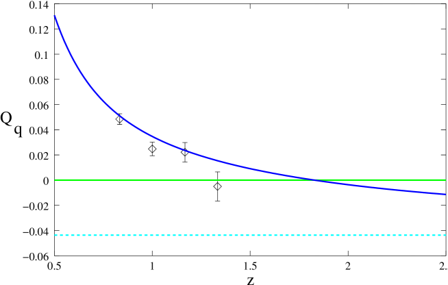
Figure 1: Comparison between free string prediction and Monte Carlo data for $Q_{q}(R)$ as defined in Eq.(24). The Monte Carlo data are taken at $\beta=0.73107$ and $T=T_{c}/3=(12a)^{-1}$, and are plotted as a function of $z=2R/L$. The solid line is the prediction Eq.(25) for this quantity. The dashed line is the asymptotic value $-\pi/6L$ of the free string prediction for large $z$.

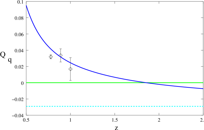
Figure 2: Same as Fig. 1 for $\beta=0.74603$ and $T=T_{c}/3=(18a)^{-1}$

A few interesting things can be learned by looking at these figures:

• The data we can use for the comparison are all in the region $z\sim 1$. This is unavoidable since small values of $z$ correspond to distances smaller than the width of the flux tube, as explained above, while data at large $z$ have large statistical uncertainties.

• In this region the free string prediction is very far from its asymptotic behavior for large $R$, where it approaches the constant

  $$F_{q}(R+1,L)-F_{q}(R,L)\to-\frac{(d-2)\pi}{6L}$$ (27)

  shown for comparison in the figures: the string correction for $z\sim 1$ has actually the opposite sign with respect to its asymptotic behavior.

• The function $F_{q}(z\equiv 2R/L)$ has a zero in $z\sim 1.8$. This is due to the fact that the asymptotic term $\pi/(6L)$ and the subdominant logarithmic term that appears in Eq.(10) have opposite signs. This in turns makes the string corrections much harder to detect in the Polyakov loop correlation functions than in the Wilson loop case, where no such cancellation occurs.

3.4 Results at $T\sim T_{c}/2$: the interacting string.

If the same comparison between Monte Carlo data and free string predictions is performed at temperatures closer to the deconfinement one, significant discrepancies begin to appear, showing that the free string contribution is not sufficient to account for the quantum fluctuations of the flux tube at such temperatures: string interaction effects, or more precisely the self-interaction of the world-sheet fields describing the string configuration, become non negligible.

The simplest way to estimate the effect of these self-interactions is to assume a Nambu-Goto action for the effective string. On one hand, this is exactly the assumption that leads one to the remarkably successful predictions Eqs.(13,14). On the other hand this same choice of string action accurately describes the string interaction effects for fluctuating interfaces in three-dimensional statistical models[23, 25].

From this assumption, one can compute the string partition function to next-to-leading order in the dimensionless expansion parameter $(\sigma RL)^{-1}$, with the choice of boundary conditions relevant to the Polyakov loop correlation function, namely Dirichlet on the two loops and periodic in the Euclidean time direction. This calculation was performed in Ref. [26] using $\zeta$-function regularization; it can be shown [27] that the same result is obtained with several other choices of regularization.

Including these contribution the string free energy Eq.(7) becomes

$$F_{q}^{(NLO)}(R,L)=(d-2)\left[\log\eta(\tau)-\frac{\pi^{2}L}{1152\ \sigma R^{3}}\left[2E_{4}(\tau)-E_{2}^{2}(\tau)\right]\right]+O\left(\frac{1}{\left(\sigma LR\right)^{2}}\right)$$ (28)

where $E_{2}$ and $E_{4}$ are the Eisenstein functions. The latter can be expressed in power series:

$$E_{2}(\tau) = 1-24\sum_{n=1}^{\infty}\sigma(n)q^{n}$$ (29)

$$E_{4}(\tau) = 1+240\sum_{n=1}^{\infty}\sigma_{3}(n)q^{n}$$ (30)

$$q \equiv e^{2\pi i\tau}$$ (31)

where $\sigma(n)$ and $\sigma_{3}(n)$ are, respectively, the sum of all divisors of $n$ (including 1 and $n$), and the sum of their cubes. The modular transformation properties

$$E_{2}(\tau) = -\left(\frac{i}{\tau}\right)^{2}E_{2}\left(-\frac{1}{\tau}\right)+\frac{6i}{\pi\tau}$$ (32)

$$E_{4}(\tau) = \left(\frac{i}{\tau}\right)^{4}E_{4}\left(-\frac{1}{\tau}\right)$$ (33)

are also useful. Note that the inclusion of next-to-leading terms does not require the introduction of any new free parameter, so that the predictive power is the same as for the free string case.

In Figs. 3-4 we show the Monte Carlo data for the string fluctuation contribution defined in Eq.(24) for $T=T_{c}/2$ compared to both the free string prediction and the Nambu-Goto string at next-to-leading order Eq.(28). We can see that Eq.(28) accurately describes the deviations of the data from the free string picture.

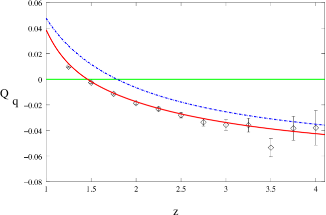
Figure 3: Data for $Q_{q}$ at $\beta=0.73107$ and $T=T_{c}/2=(8a)^{-1}$. The solid line is the full NLO string prediction, while the dash-dotted line is the free string prediction.

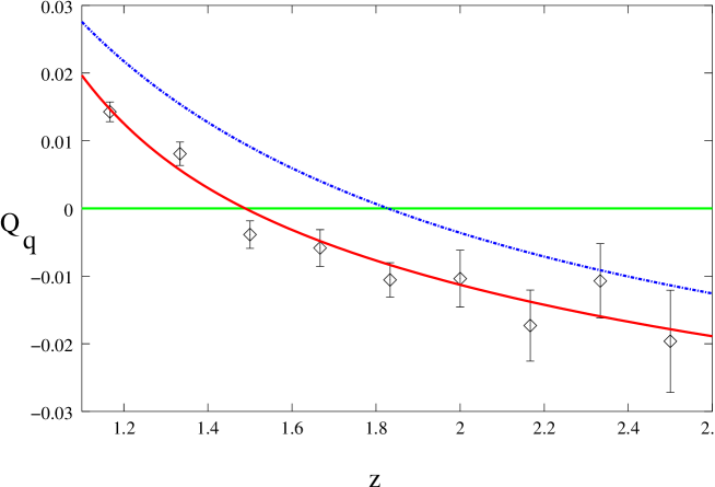
Figure 4: Same as Fig. 4 for $\beta=0.74603$ and $T=T_{c}/2=(12a)^{-1}$

A word of caution is however in order: while the free string prediction Eq.(7) is the universal infrared limit of a large class of interacting string models (see e.g. the various models considered in [26]), the interaction contributions depend on the choice of the model. Therefore while the validity of the free string model in the infrared limit $R,L\to\infty$ is basically a consequence of the masslessness and bosonic character of the fields describing the string fluctuations, the choice of the Nambu-Goto action is a much stronger statement, that cannot as far as we know be based on simple physical grounds. Nevertheless, it is certainly noteworthy that the same choice of action gives accurate predictions for fluctuating interfaces [23, 25] and Polyakov loop correlation functions.

4 Conclusions

The study of Polyakov loop correlation functions in the three-dimensional $\mathbb{Z}_{2}$ model allows us to gain some insight on the effect of the fluctuations of the confining flux tube, which is likely to be relevant also in more complicated and realistic gauge theories. The main points we have elucidated are:

1. The quantum fluctuations of the confining string give a computable and numerically relevant contribution to the Polyakov loop correlation functions in the confined phase.

2. The free bosonic string model describes well such contributions provided the temperature $T$ is not too close to the critical one: in our case $T\leq T_{c}/3$ is required to find good agreement.

3. When the temperature gets closer to $T_{c}$, next-to-leading effects in the string partition function become important. Assuming a Nambu-Goto action for the confining string one can compute these effects and find excellent agreement with the Monte Carlo data also at $T\sim T_{c}/2$.

Acknowledgement

We would like to thank M. Hasenbusch for reading a previous version of this work and offering several useful suggestions.

References

- [1] M. Luscher, K. Symanzik and P. Weisz, “Anomalies Of The Free Loop Wave Equation In The Wkb Approximation,” Nucl. Phys. B 173 (1980) 365.
- [2] M. Luscher, “Symmetry Breaking Aspects Of The Roughening Transition In Gauge Theories,” Nucl. Phys. B 180 (1981) 317.
- [3] M. Caselle, R. Fiore, F. Gliozzi, M. Hasenbusch and P. Provero, “String effects in the Wilson loop: A high precision numerical test,” Nucl. Phys. B 486 (1997) 245 [arXiv:hep-lat/9609041].
- [4] M. Caselle, R. Fiore, F. Gliozzi, P. Provero and S. Vinti, “String Contributions In 3-D Z(2) And Z(5) Gauge Models,” Int. J. Mod. Phys. A 6 (1991) 4885.
- [5] M. Caselle, R. Fiore, F. Gliozzi and S. Vinti, “The Effective string of 3-D Z(2) gauge theory as a c = 1 compactified CFT,” Int. J. Mod. Phys. A 8 (1993) 2839 [arXiv:hep-lat/9207001].
- [6] M. Caselle, F. Gliozzi, U. Magnea and S. Vinti, “Width of Long Colour Flux Tubes in Lattice Gauge Systems,” Nucl. Phys. B 460 (1996) 397 [arXiv:hep-lat/9510019].
- [7] S. Necco and R. Sommer, “The N(f) = 0 heavy quark potential from short to intermediate distances,” Nucl. Phys. B 622 (2002) 328 [arXiv:hep-lat/0108008].
- [8] B. Lucini and M. Teper, “Confining strings in SU(N) gauge theories,” Phys. Rev. D 64 (2001) 105019 [arXiv:hep-lat/0107007].
- [9] F. Gliozzi and P. Provero, Nucl. Phys. B 556 (1999) 76 [arXiv:hep-lat/9903013].
- [10] M. Minami, “How ’Can One Hear The Shape Of A Drum’ In The Dual Partition Functions?,” Prog. Theor. Phys. 59 (1978) 1709.
- [11] P. de Forcrand, G. Schierholz, H. Schneider and M. Teper, “The String And Its Tension In SU(3) Lattice Gauge Theory: Towards Definitive Results,” Phys. Lett. B 160 (1985) 137.
- [12] M. Flensburg and C. Peterson, “String Model Potentials And Lattice Gauge Theories,” Nucl. Phys. B 283 (1987) 141.
- [13] R. D. Pisarski and O. Alvarez, “Strings At Finite Temperature And Deconfinement,” Phys. Rev. D 26 (1982) 3735.
- [14] P. Olesen, “Strings, Tachyons And Deconfinement,” Phys. Lett. B 160 (1985) 408.
- [15] M. Hasenbusch and K. Pinn, “Computing the Roughening Transition of Ising and Solid-On-Solid Models by BCSOS Model Matching,” J. Phys. A 30 (1997) 63 [arXiv:cond-mat/9605019].
- [16] H. W. Blote, L. N. Shchur and A. L. Talapov, “The Cluster Processor: New Results,” Int. J. Mod. Phys. C 10 (1999) 1137-1148 [arXiv:cond-mat/9912005].
- [17] M. Caselle and M. Hasenbusch, “Deconfinement transition and dimensional cross-over in the 3D gauge Ising model,” Nucl. Phys. B 470 (1996) 435 [arXiv:hep-lat/9511015].
- [18] M. Creutz, “Microcanonical Monte Carlo Simulation,” Phys. Rev. Lett. 50 (1983) 1411.
- [19] G. Bhanot, M. Creutz and H. Neuberger, “Microcanonical Simulation Of Ising Systems,” Nucl. Phys. B 235 (1984) 417.
- [20] K. Rummukainen, “Multicanonical cluster algorithm and the 2-D seven state Potts model,” Nucl. Phys. B 390 (1993) 621 [arXiv:hep-lat/9209024].
- [21] V. Agostini, G. Carlino, M. Caselle and M. Hasenbusch, “The spectrum of the 2+1-dimensional gauge Ising model,” Nucl. Phys. B 484 (1997) 331 [arXiv:hep-lat/9607029].
- [22] M. Hasenbusch and K. Pinn, “Surface tension, surface stiffness, and surface width of the three-dimensional Ising model on a cubic lattice,” PhysicaA 192 (1993) 342 [arXiv:hep-lat/9209013].
- [23] M. Caselle, R. Fiore, F. Gliozzi, M. Hasenbusch, K. Pinn and S. Vinti, “Rough interfaces beyond the Gaussian approximation,” Nucl. Phys. B 432 (1994) 590 [arXiv:hep-lat/9407002].
- [24] M. Hasenbusch and K. Pinn, “The interface tension of the 3D Ising model in the scaling region” Physica A 245 (1997) 366 [arXiv:cond-mat/9704075].
- [25] P. Provero and S. Vinti, “Capillary Wave Approach To Order-Order Fluid Interfaces In The 3-D Three State Potts Model,” PhysicaA 211 (1994) 436 [arXiv:hep-lat/9310028].
- [26] K. Dietz and T. Filk, “On The Renormalization Of String Functionals,” Phys. Rev. D 27 (1983) 2944.
- [27] M. Caselle and K. Pinn, “On the Universality of Certain Non-Renormalizable Contributions in Two-Dimensional Quantum Field Theory,” Phys. Rev. D 54 (1996) 5179 [arXiv:hep-lat/9602026].