Connections between Thin,Thick and Projection Vortices in SU(2) Lattice Gauge Theory

Abstract

We elucidate the connection between $SO(3)\times Z(2)$ and the usual $SU(2)$ configuration variables. By exploiting the freedom of choosing a particular $SO(3)$ representative we find a direct connection between the two configuration spaces. We are then able to compare the Kovacs-Tomboulis formulation of center vortices with the projection vortex formulation on the same configuration. Choosing a different representative, and going to the maximal center gauge, we show that projection vortices occur without approximation. The projection vortex dominance approximation results from dropping a factor in an exact expression for the Wilson loop.

1 Introduction

In the interest of finding a precise definition of thick center vortices on the lattice, Tomboulis[1] and later Tomboulis and Kovacs[2] reformulated SU(2) gauge theory in terms of variables defined on the factor groups $SO(3)$ and $Z(2)$. The partition function and operators expressed in these variables are invariant under a sign flip of each link. A particular choice of the sign of the trace of each link variable corresponds to the choice of a representative of $SO(3)$. The bookkeeping that preserves the SU(2) theory is provided by new Z(2) valued plaquette variables forming closed thin vortices. A sign flip of a link forming a Wilson loops is accompanied by the introduction of a vortex linked to it giving a compensating tiling factor of $-1$.

In a recent paper[3] we found a direct kinematical connection between this approach and the usual SU(2) formalism. For a particular $SO(3)$ representative the two formulations are identical. Therefore we can define both the Kovacs-Tomboulis[2] (KT) and the Projection (P) vortex counters[4] on the same configuration giving a direct comparison of these two approaches.

Secondly, by choosing another $SO(3)$ representative we showed that the resulting thin vortices are precisely the structures known as P vortices. The projection approximation comes from a subsequent truncation.

Although the $SO(3)\times Z(2)$ formulation is equivalent to the $SU(2)$ form, the former is particularly useful in illustrating connections between the KT and P vortex approaches. Configurations are generated most efficiently in the SU(2) variables. One can match the $SU(2)$ variables to the corresponding $SO(3)\times Z(2)$ variables. Then we are free to flip the signs of the links thereby changing representative. If one chooses signs for which the trace of all links are positive, then the thin vortices created in the process will be identical to the those generaged by the projection algorithm[4].

In the $SO(3)\times Z(2)$ formulation, Wilson loops have a perimeter factor and a tiling factor. Changing the representative may move a minus sign from one factor to another, but always leaves the product invariant. This separation is gauge dependent. The goal of the projection approach is to transfer the disordering from the perimeter factor to the tiling factor since the the projection approximation consists of setting the perimeter factor to one. The quality of the P vortex approximation then depends on one’s ability to suppress the disordering mechanism in the perimeter factor through a judicious choice of gauge[6, 7, 8, 9, 10, 11].

2 $SU(2)$ configurations in $SO(3)\times Z(2)$ variables

The Wilson form of the partition function can be recast by introducing $Z(2)$ valued independent variables $\sigma(p)$ defined on plaquettes[1, 5]

$$Z_{SO(3)\times Z(2)} = \int\left[dU(b)\right]\sum_{\sigma(p)}$$

$$\left[\prod_{c}\delta\left(\sigma(\partial c)\eta(\partial c)\right)\right]$$

$$\exp\left(\beta\sum_{p}\frac{1}{2}|Tr[U(\partial p)]|\sigma(p)\right),$$

where the dependent variables $\eta(p)$ are defined by

$$Tr[U(\partial p)]\equiv|Tr[U(\partial p)]|\eta(p).$$

The “cube constraint” factor requires that $\prod_{1}^{6}\eta(p)\sigma(p)=+1$ over the six faces of all cubes.

Wilson loops have $Z(2)$ valued plaquette tiling factors, $\sigma$ and $\eta$ on an arbitrary surface $S$ bounded by $C$

$$W_{m\times n}(C) = \hbox{\small Tr}[U(C)]\eta(S)\sigma(S)|_{C=\partial S},$$ (1)

$$W_{1\times 1} = \hbox{\small Tr}[U(\partial p)]\eta(p)\sigma(p)=|\hbox{\small Tr}[U(\partial p)]|\sigma(p).$$

Properties of this form include:

• $Z(2)$ invariance of $Z$ and of observables under $U(b)\rightarrow-U(b)$. There are therefore $2^{N}$ representatives of $SO(3)$, where $N$ is the number of links.
  

• There exist co-closed $\sigma(p)-\eta(p)$ vortex sheets due to the cube constraint with patches of either $\sigma(p)=-1$ or $\eta(p)=-1$, $\sigma(p)\eta(p)=-1$. Pure $\sigma(p)$ or $\eta(p)$ vortex sheets are limiting cases.
  

• A change of representative can deform existing $\eta$ patches and create or destroy pure $\eta$ vortex sheets.

2.1 The representative $\widetilde{U}$

This is defined by the condition

$$\sigma(p)\eta(p) = +1,\;\;\;\forall p.$$

In this case the cube constraint is automatically satisfied. There are further simplifications:

$$|Tr[\widetilde{U}(\partial p)]|\sigma(p) = Tr[\widetilde{U}(\partial p)]\eta(p)\sigma(p),$$

$$= Tr[\widetilde{U}(\partial p)],$$

$$\widetilde{Z} = \int\left[d\widetilde{U}(b)\right]\exp\left(\beta\sum_{p}\frac{1}{2}\hbox{\small Tr}[\widetilde{U}(\partial p)]\right),$$

$$W_{m\times n}=\hbox{\small Tr}[\widetilde{U}(C)],\;\;W_{1\times 1}=\hbox{\small Tr}[\widetilde{U}(\partial p)].$$

We showed[5, 3] that starting from a cold configuration, $U(b)=\sigma(p)=+1$, we can reach the full configuration space of the independent variables $\{U(b),\sigma(p)\}$ through local updates while staying in the representative $\widetilde{U}(b)$. In this representative all $\sigma-\eta$ vortices are absent.

This particular representative provides the connection of this formulation to the SU(2) formalism with the Wilson action. As a consequence, we can define the Tomboulis thin, thick and hybrid vortex counters on ordinary $SU(2)$ configurations as will be given below.

2.2 The representative $\widehat{U}$

This is defined by the condition

$$\hbox{\small Tr}[\widehat{U}(b)] \geq 0.$$

This can be obtained by a single sweep. The interest in this is to connect with P vortices which are defined as follows: One first fixes the gauge, for example the maximal center gauge and then

In an arbitrary representative

• Project: $sign\hbox{\small Tr}[U(b)]\rightarrow u(b)$, $u(b)=\pm 1$.

• $P$ vortex: $u(p)=u(\partial p)\eta(p)\sigma(p)=-1$

• Proj. approx.: $W(C)\approx u(S)|_{C=\partial S}$.

In the $\widehat{U}(b)$ representative

• Project: $sign\hbox{\small Tr}[\widehat{U}(b)]\rightarrow\widehat{u}(b)$, $\widehat{u}(b)=+1$.

• $P$ vortex: $\widehat{u}(p)=\eta(p)\sigma(p)=-1$, which is identical to $\sigma-\eta$ vortex.

• Proj. approx.: $\hbox{\small Tr}[\widehat{U}(C)]\approx 1$,

where we have used Eqn.(1). These two procedures give identical P vortices.

However in the $\widehat{U}(b)$ representative the $P$ vortices are identical to the $\sigma-\eta$ vortices which are a tiling factor in the exact definition of the Wilson loop. The success or failure of a projection approximation depends on whether one can find a gauge such that the sign fluctuations of the perimeter factor in Eqn.(1) can be transferred to the tiling factors arising from $\sigma-\eta$ linkages. If so then one argues that the area law of a Wilson loop arises from P vortex linkages in that gauge.

3 Kovacs-Tomboulis vortex counters

Kovacs and Tomboulis[2] gave representative independent definitions of three vortex counters based on $SO(3)\times Z(2)$ configurations.

$$N_{thin}(S) = \prod_{p\in S}\sigma(p),$$

$$N_{thick}(S) = \hbox{\small sign}\;\hbox{\small tr}[U(C)]\times\prod_{p\in S}\eta(p),$$

$$N_{hybrid}\;\;\;\; = N_{thin}(S)\times N_{thick}(S)=\hbox{\small sign}\,W.$$

The hybrid counter is necessarily independent of surface. $N_{thin}(S)$ and $N_{thick}(S)$ count the corresponding vortices only if the value is independent of surface $S$.

We can express these counters in terms of $SU(2)$ configurations by evaluating the above expressions in the $\widetilde{U}(b)$ representative.

$$N_{thin}(S) = \prod_{p\in S}\hbox{\small tr}[\partial\widetilde{U}(p)],$$

$$N_{hybrid}\;\;\;\; = \hbox{\small sign}\,\,\hbox{\small tr}[\widetilde{U}(C)],$$

$$N_{thick}(S) = \prod_{p\in S}\hbox{\small sign}\,\,\hbox{\small tr}[\partial\widetilde{U}(p)]\times\hbox{\small sign}\,\,\hbox{\small tr}[\widetilde{U}(C)].$$

4 Numerical Results

It is not feasible to measure these counters on all possible surfaces. We made measurements only on the minimal surface[3, 5]. As a consequence, a measurement giving for example $N_{thin}(S)=-1$ indicates only the occurrence of an odd number of $\sigma$ patches which could be part of thin or hybrid vortices. And similarly for the thick case.

The contribution to the potential from the three types of vortex counters is

$$V(R)=-\lim_{T\rightarrow\infty}\frac{1}{T}\ln\langle N(W(R,T))\rangle,$$

where $N(W(R,T))$ is the thin, thick or hybrid counter signal for that particular Wilson loop (taking values $\pm 1$).

Fig. 1 shows that the string tension in $V_{thin}$ in physical units increases in the approach to the continuum limit. Although this is perhaps surprising, we showed that this is canceled by an increasing string tension in the thick potential[3].

The K-T definition for vortices[2] is appealing since it is gauge invariant but they are hard to localize on a lattice. P vortices[4], on the other hand, are easy to localize but are not gauge invariant. It is interesting to see if these two definitions agree. We now have the tools to compare these definitions of vortex counters on the same configuration.

Fig. 2 shows plots of the average of the fraction odd/(odd+even) hybrid and P vortices linking a Wilson loop as a function of area. The average of the product compared to the product of the average shows that there is essentially no correlation. The corresponding plots for thin vortex fractions and thick ones gives essentially the same result. In Ref.[3] we examine more sensitive signals of correlations but without a definitive result.

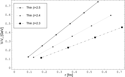
Figure 1: Vortex potentials in physical units for the thin counter.

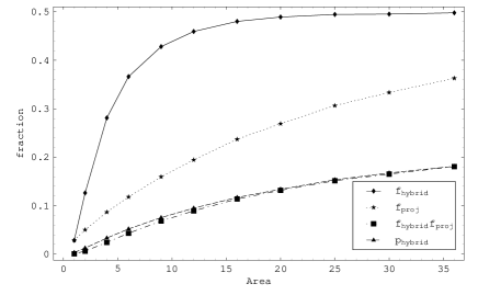
Figure 2: Average of the fraction odd/ (odd+even) hybrid and projection vortices linking a Wilson loop as a function of area.

5 Idealized vortex configurations

As we see from the numerical results it is problematic to assign the same physics to the KT and P vortex counters because of the absence of a simple correlation. To understand the reasons for this it may be a useful exercise to look at an idealized configuration for which the two approaches give the same signal. We are thinking of the situation in which center vortices are well defined and isolated from one another by regions of pure gauge. We denote the domain of pure gauge by ${\cal D}$ for which all links are gauge equivalent to $\pm I$ and a complementary domain in which the field strength may be non-zero. Assume in general that ${\cal D}$ is multiply connected.

Go to the gauge where all links in ${\cal D}$ $=\pm I$. The advantage of the $SO(3)\times Z(2)$ variables is that we can subsequently go to the representative such that all links in ${\cal D}$ $=+I$. Consider a Wilson loop in this multi-connected region ${\cal D}$. The perimeter factor $=+1$. The tiling factors are due to the thin vortices linked to the loop.

KT interpretation

Center vortices are defined only by their topological linkage. The linkage is unambiguous only if the perimeter of the loop is completely in the domain ${\cal D}$. The value of the loop in this case is determined by the tiling factor alone which counts thin $\eta-\sigma$ vortex linkages, $\hbox{\small mod}(2)$. If there are $\sigma$ patches present in the $\eta-\sigma$ vortex, then the thick vortex degenerates to a thin vortex at those locations but in general spreads out forming a thick vortex elsewhere. KT refers to this as a hybrid vortex.

P interpretation

The construction has fixed the positions of the P vortices. One can locate and count those linking the loop giving a factor of $(-1)^{n}$ for the Wilson loop for the case of $n$ vortices.

Comparison

The two approaches arrive at the same value for the Wilson loop on this idealized configuration. The P and $\eta-\sigma$ vortices are the same. Both approaches come to the same conclusion on the presence or absence of a bona fide center vortex, mod($2$). However the KT definition is gauge invariant and representative invariant and therefore any particular details in this gauge and this representative such as location of the thin vortices is not particularly relevant. The P vortices are fixed by the construction and the pattern could indicate a substructure. However identifying substructure center vortices can not be tested by the KT topological definition if it involves a Wilson loop perimeter that strays from the domain ${\cal D}$.

If this simple picture has some validity, the numerical results suggests that it is obscured by noise in the domain ${\cal D}$ and/or vortex cores that overlap, among many other possibilities. It might be helpful if one could find a related theory in which the dynamics creates vortices on one time scale establishing their identity and the vortices move and deform on longer time scale.

6 Summary and Conclusions

We have shown that

• An $SO(3)\times Z(2)$ configuration is identical to an $SU(2)$ configuration in a particular representative. Updates of the former can be done with the simpler $SU(2)$ variables.

• The $\eta-\sigma$ vortices of Kovacs and Tomboulis are identical to P vortices in an particular gauge and a particular representative.

• The KT vortex counters are gauge invariant and representative invariant and are measurable on $SU(2)$ configurations.

• The string tension due to $\sigma$ patches of thin vortices taken alone has a surprising and definitive signal of increasing string tension as $a\rightarrow 0$. The thick patches behave similarly and taken together, the scaling violations cancel.

• A simple test for correlations of KT and P vortex counters gives a null result. More sensitive tests have been reported elsewhere[3] but without definitive results.

7 Acknowledgments

This work was supported in part by the United States Department of Energy, grant DE-FG05-91 ER 40617.

References

- [1] Tomboulis, E.T. (1981) ’tHooft loop in lattice gauge theories, Phys. Rev. D23, 2371-2383.
- [2] Kovacs, T.G., and Tomboulis, E.T. (1998) Vortices and confinement at weak coupling, Phys. Rev. D 57, 4054-4062.
- [3] Alexandru, A., and Haymaker, R.W. (2001), Center vortices on lattices, Phys. Lett. B 520, 410-420.
- [4] Del Debbio, L., Faber, M., Greensite, J. and Olejnik, S. (1997), Center Dominance and Z2 Vortices in SU(2) Lattice Gauge Theory, Phys. Rev. D 55, 2298.
- [5] Alexandru, A. and Haymaker, R.W. (2000), Vortices in simulations, Phys. Rev. D62, 074509-1-13.
- [6] Del Debbio,L., Faber, M., Giedt, J., Greensite, J. and Olejnik, S. (1998), Detection of Center Vortices in the Lattice Yang-Mills Vacuum, Phys. Rev. D 58, 094501-1-28.
- [7] Kovacs, T. G. and Tomboulis, E. T. (1999), On P-vortices and the Gribov problem, Phys. Lett. B 463, 104-108.
- [8] Bornyakov, V. G., Komarov, D. A., Polikarpov, M. I. and Veselov, A. I. (2000), P-vortices, nexuses and effects of gauge copies, JETP Lett. 71, 231-234.
- [9] Bertle,R., Faber, M., Greensite, J. and Olejnik, S. (2000), P-Vortices, Gauge Copies, and Lattice Size, JEHP 0010, 007.
- [10] Bornyakov, V. G., Komarov, D. A. and M.I. Polikarpov (2001), P-vortices and Drama of Gribov Copies, Phys. Lett. B 479, 151-158.
- [11] Faber, M., Greensite, J. and Olejnik, S. (2002), Center dominance recovered: Direct Laplacian center gauge, Nucl. Phys. B (Proc. Suppl.) 106, 652-654.