Abstract

We review arguments for center dominance in center gauges where vortex locations are correctly identified. We introduce an appealing interpretation of the maximal center gauge, discuss problems with Gribov copies, and a cure to the problems through the direct Laplacian center gauge. We study correlations between direct and indirect Laplacian center gauges.

1 Why Center Dominance?

The aim of most lattice studies of the confinement mechanism is to extract from lattice link variables the most relevant parts for the infrared dynamics. The concept of (some kind of) dominance seems a necessary, though not sufficient, condition for success. If we extract the (would-be) relevant parts of links and compute physical quantities related to confinement (e.g. the string tension) we expect to reproduce their behavior in the full theory. Were it not the case, one could hardly claim to have achieved the goal.

It was observed both in SU(2) [1, 2] and (less convincingly) in SU(3) lattice gauge theory [3] that the string tension obtained from center-projected configurations in maximal center gauge (MCG) agrees remarkably well with the asymptotic string tension of the full theory. This phenomenon of center dominance has led to the recent revival of interest in the center-vortex picture of color confinement [4, 5, 6]. One can easily formulate an argument why center dominance should occur if center vortices are correctly identified [2]:

Vortices are created by discontinuous gauge transformations. Let a closed loop $C$, parametrized by $x^{\mu}(\tau)$, $\tau\in[0,1]$, encircle $n$ vortices. At the point of discontinuity (in SU(2)):

$$g(x(0))=(-1)^{n}g(x(1)).$$ (1)

The corresponding vector potential in the neighborhood of $C$ can be decomposed as

$$A^{(n)}_{\mu}(x)=g^{-1}\delta A^{(n)}_{\mu}(x)g+ig^{-1}\partial_{\mu}g.$$ (2)

The $g^{-1}\partial_{\mu}g$ term is dropped at the discontinuity. Then, the value of the Wilson loop is

$$W_{n}(C)=\langle\mbox{Tr}\exp[i\oint dx^{\mu}A_{\mu}^{(n)}]\rangle=(-1)^{n}\langle\mbox{Tr}\exp[i\oint dx^{\mu}\delta A_{\mu}^{(n)}]\rangle.$$ (3)

In the region of the loop $C$, the vortex background looks locally like a gauge transformation. If all other fluctuations $\delta A^{(n)}_{\mu}$ are basically short-range, then they should be oblivious, in the neighborhood of the loop $C$, to the presence or absence of vortices in the middle of the loop. In that case:

$$\langle\mbox{Tr}\exp[i\oint dx^{\mu}\delta A_{\mu}^{(n)}\rangle\approx\langle\mbox{Tr}\exp[i\oint dx^{\mu}\delta A_{\mu}^{(0)}]\rangle$$ (4)

for sufficiently large loops, and therefore

$${W_{n}(C)/W_{0}(C)}\longrightarrow(-1)^{n}\quad\mbox{or}\quad W(C)\approx Z(C)\times\langle\mbox{Tr}\exp[i\oint dx^{\mu}\delta A_{\mu}^{(0)}]\rangle.$$ (5)

Here $W(C)$ is the expectation value of the full Wilson loop, and $Z(C)$ the expectation value of the loop constructed from center elements alone.

It is clear from the above argument that one gets center dominance, i.e. the same string tension from $W(C)$ and $Z(C)$, under four intertwined assumptions:

1. Vortices are the confinement mechanism.

2. Vortices are correctly identified.

3. Short-range fluctuations with/without vortices look similar.

4. No area law arises from the last factor in Eq. (5).

Is there a necessity to fix any gauge? The original vortex idea was formulated without a reference to a particular gauge, and in fact a kind of center dominance exists even without gauge fixing, as was shown in [7]. However, this holds for any distances, not only for large ones, vortices defined without gauge fixing do not fulfill simple expectations and do not scale according to the renormalization group, and thus the phenomenon hardly bears any information on the confinement mechanism. Gauge fixing appears of special importance for correct identification of vortices.

2 How to Identify Center Vortices?

The procedure, proposed in [1, 2], consists of three steps:

1. Fix thermalized SU(2) lattice configurations to direct maximal center (or adjoint Landau) gauge by maximizing the expression:

   $$\sum_{x,\mu}\;\Bigl{|}\mbox{Tr}[U_{\mu}(x)]\Bigr{|}^{2}\;\qquad\mbox{or equivalently}\qquad\sum_{x,\mu}\;\mbox{Tr}[U^{A}_{\mu}(x)]\;.$$ (6)

2. Make center projection by replacing:

   $$U_{\mu}(x)\rightarrow Z_{\mu}(x)\equiv\mbox{sign Tr}[U_{\mu}(x)]\;.$$ (7)

3. Finally, identify excitations (P-vortices) of the resulting $Z_{2}$ lattice configurations.

A whole series of results, obtained by our and other groups, indicates that center vortices defined in MCG play a crucial role in the confinement mechanism. This includes, besides center dominance, the following:

1. P-vortices locate center vortices in full lattice configurations [2].

2. P-vortices locate physical objects, their density scales according to the renormalization group [8].

3. Creutz ratios computed from center-projected Wilson loops are almost constant starting from shortest distances; the Coulomb contribution was effectively eliminated (precocious linearity) [2].

4. Center vortices are correlated not only with confinement, but with chiral symmetry breaking and non-trivial topology as well [9].

5. Deconfinement can be understood as a center vortex percolation transition [10, 11].

Other gauges work as well; general conditions a suitable gauge has to fulfill were formulated in [12]. Here we would just like to briefly summarize an interesting insight into the meaning of MCG fixing and center projection, due to [13, 14].

3 Best-fit Interpretation of MCG

Running a MC simulation, one can ask for the pure gauge configuration closest, in configuration space, to a given lattice gauge field:

$$U_{\mu}(x)\quad\sim\quad g(x)g^{\dagger}(x+\hat{\mu})\equiv U_{\mu}^{(0)}(x).$$ (8)

It is easy to show that finding the optimal $g(x)$ is equivalent to the problem of fixing to the Landau gauge.

Let us now allow for $Z_{2}$ dislocations in the gauge transformation, i.e. fit the lattice configuration by a thin center vortex configuration:

$$U_{\mu}^{vor}(x)\equiv g(x)Z_{\mu}(x)g^{\dagger}(x+\hat{\mu}),\qquad Z_{\mu}(x)=\pm 1$$ (9)

$U_{\mu}^{vor}(x)$ becomes a continuous pure gauge in the adjoint representation, blind to the $Z_{\mu}(x)$ factor. One can make the fit in two steps:

1. Determine $g(x)$ up to a $Z_{2}$ transformation by minimizing the square distance $d^{2}_{A}$ between $U_{\mu}$ and $U_{\mu}^{vor}$ in the adjoint representation, which is easily seen to be equivalent to fixing to direct MCG.

2. Find $Z_{\mu}(x)$ by minimizing:

$$\mbox{Tr}\Bigl{\{}\left[U_{\mu}(x)-g(x)Z_{\mu}(x)g^{\dagger}(x+\hat{\mu})\right]\left[U_{\mu}^{\dagger}(x)-g(x+\hat{\mu})Z_{\mu}(x)g^{\dagger}(x)\right]\Bigr{\}},$$ (10)

which requires the center projection prescription, Eq. (7).

Summarizing, the procedure of direct MCG fixing + center projection represents the best fit of a lattice configuration by a set of thin center vortices.

4 Why Does MCG Sometimes Fail to Find Vortices?

MCG fixing suffers from the Gribov copy problem. The iterative gauge-fixing procedure converges to a local maximum which will be slightly different for every gauge copy of a given lattice configuration.

At the first sight, the problem seemed quite innocuous: We observed in [2] that vortex locations in random copies of a given configuration were strongly correlated. However, the successes of the approach were seriously questioned. Bornyakov et al. [15] showed that using the method of simulated annealing instead of our usual (over-)relaxation, one could find better (local) MCG maxima, but the center-projected string tension was only about 2/3 of the full one.

The best-fit interpretation of the previous section provides us with a clue to the origin of this problem. It is clear that $U_{\mu}^{vor}(x)$ is a bad fit to $U_{\mu}(x)$ at links belonging to thin vortices (i.e. to the P-plaquettes formed from $Z_{\mu}(x)$). We recall that a plaquette $p$ is a P-plaquette iff $Z(p)=-1$ (where $Z(C)$ denotes the product of $Z_{\mu}(x)$ around the contour $C$) and that P-plaquettes belong to P-vortices. Let us write the gauge transformed configuration as

$${}^{g}U_{\mu}(x)=Z_{\mu}(x)\;e^{iA_{\mu}(x)},\qquad\mbox{Tr}\;e^{iA_{\mu}(x)}\geq 0.$$ (11)

At large $\beta$ values $\textstyle{\frac{1}{2}}\mbox{Tr}[U_{P}]=1-O(1/\beta)$, and equals to

$$\left(Z_{P}\right)\textstyle{\frac{1}{2}}\mbox{Tr}\displaystyle{\prod_{P}}e^{iA_{\mu}(x)}={}_{~{}\atop\mbox{{\small\it on P-plaquettes\ }}}{(-1)}\times\textstyle{\frac{1}{2}}\mbox{Tr}\displaystyle{\prod_{P}}e^{iA_{\mu}(x)}.$$ (12)

The last equation implies that at least at one link belonging to the P-plaquette $A_{\mu}(x)$ cannot be small, therefore ${}^{g}U_{\mu}(x)$ must strongly deviate from the center element.

The above argument shows that the quest for the global maximum may not always be the best strategy; one should rather try to exclude contributions from P-plaquettes where the fit is inevitably bad  [14], or modify the gauge fixing procedure to soften the fit at vortex cores.

5 A Cure for the Disease: Direct Laplacian Center Gauge

We have recently proposed to overcome the Gribov problem using the direct Laplacian center gauge [16]. The proposal was to a large extent inspired by the Laplacian Landau [17], Laplacian abelian [18], and Laplacian center [19] gauges. The idea is the following:

To find the “best fit” to a lattice configuration by a thin center vortex configuration one looks for a matrix $M(x)$ maximizing the expression:

$${\cal{R}}_{M}=\displaystyle{\sum_{x,\mu}}\mbox{Tr}\left[M^{T}(x)U_{A\mu}(x)M(x+\hat{\mu})\right],$$ (13)

with a constraint that $M(x)$ should be an SO(3) matrix at any site $x$:

$$M^{T}(x)\cdot M(x)={\mathbf{1}},\qquad\det M(x)=1.$$ (14)

We soften the orthogonality constraint by demanding it only “on average”:

$$\langle M^{T}\cdot M\;\rangle\equiv\displaystyle{\frac{1}{\cal V}\sum_{x}}M^{T}(x)\cdot M(x)=\mathbf{1}.$$ (15)

It is convenient to write the columns of $M(x)$ as a set of 3-vectors: $f^{b}_{a}(x)=M_{ab}(x)$. The optimal $M(x)$, maximizing ${\cal{R}}_{M}$ with the constraint, is determined by the three lowest eigenvectors $f^{b}_{a}(x)$:

$${\cal D}_{ij}(x,y)f^{a}_{j}(y)=\lambda_{a}f^{a}_{i}(x)$$ (16)

of the covariant adjoint Laplacian operator ${\cal D}_{ij}(x,y)$:

$${\cal{D}}_{ij}(x,y)=\sum_{\mu}\Bigl{(}2\delta_{xy}\delta_{ij}-\left[U_{A\mu}(x)\right]_{ij}\delta_{y,x+\hat{\mu}}-\left[U_{A\mu}(x-\hat{\mu})\right]_{ji}\delta_{y,x-\hat{\mu}}\Bigr{)}.$$ (17)

The resulting real matrix field $M(x)$ has further to be mapped onto an SO(3)-valued field $g_{A}(x)$. A naive map (which could also be called Laplacian adjoint Landau gauge) amounts to choosing $g_{A}(x)$ closest to $M(x)$. Such a map is well known in matrix theory and is called polar decomposition.

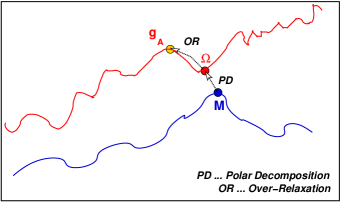
Figure 1.  : Scheme of the Laplacian mapping of $M(x)$ to a nearby SO(3) matrix field $g_{A}(x)$.

A better procedure, in our opinion, is the Laplacian map, that leads to direct Laplacian center gauge. We try to locate $g_{A}(x)$ as close to $M(x)$ local maximum of the MCG (constrained) maximization problem. To achieve this, we first make the naive map (polar decomposition), then use the usual quenched maximization (overrelaxation) to relax to the nearest (or at least nearby) maximum of the MCG fixing condition. This procedure is illustrated schematically in Fig. 1.

To test the new procedure, we have recalculated the vortex observables introduced in our previous work (cf. Refs. [1, 2]), with P-vortices located via center projection after fixing the lattice to the new direct Laplacian center gauge. The results are summarized on the following page.

The quantities of the most immediate interest are the center-projected Creutz ratios. Our data for the range of couplings $\beta=2.2-2.5$ is displayed on a logarithmic plot in Fig. 2a. In general $\chi_{cp}(R,R)$ deviates from the full asymptotic string tension by less than 10%.

(a)

(c)

(b)

(d)

(e)

Figure 2.  : Results from direct Laplacian center gauge:
(a) Combined data, at $\beta=2.2-2.5$, for center-projected Creutz ratios obtained after direct Laplacian center gauge fixing. Horizontal bands indicate the asymptotic string tensions on the unprojected lattice, with the corresponding errorbars, taken from [20].
(b) The ratio of projected Creutz ratios to the full asymptotic string tension, as a function of loop extension in fermis. The data is taken from $\chi_{cp}(R,R)$ at a variety of couplings and lattice sizes.
(c) Evidence of asymptotic scaling of the P-vortex surface density. The solid line is the asymptotic freedom prediction with $\sqrt{\rho/6\Lambda^{2}}=50$.
(d) Ratio of one- and two-vortex to zero-vortex Wilson loops $W_{1,2}(C)/W_{0}(C)$ vs. loop area, at $\beta=2.3$ on a $16^{4}$ lattice.
(e) Creutz ratios on the modified lattice, with vortices removed, at $\beta=2.3$.

As another way of displaying both center dominance and precocious linearity, we show, in Fig. 2b, the ratio

$${\chi_{phys}(R,R)/\sigma_{phys}}={\chi_{cp}(R,R)/\sigma_{Lat}(\beta)}$$ (18)

as a function of the distance in physical units $R_{phys}=Ra(\beta)$ for all $\chi_{cp}(R,R)$ data points taken in the range of couplings $\beta=2.3-2.5$. Again we see that the center-projected Creutz ratios and asymptotic string tension are in good agreement (deviation $<10\%$), and there is very little variation in the Creutz ratios with distance. We should probably stress in this context the significance of precocious linearity: it implies that center-projected degrees of freedom have isolated the long-range physics, and are not mixed up with ultraviolet fluctuations.

Other encouraging results from MCG are recovered in the new gauge as well. Figure 2c shows the P-vortex density vs. $\beta$ in a logarithmic plot. The density scales according to the asymptotic freedom formula with the slope corresponding to a quantity that behaves like a surface density. The slope for pointlike objects (like instantons), or linelike objects (like monopoles) would be quite different.

Figure 2d presents the data on vortex-limited Wilson loops. One can clearly see the expected trend, see Eq. (5), for large enough loops. Figure 2e shows that removal of center vortices causes the asymptotic string tension to vanish.

6 How Does DLCG Differ from Laplacian Center Gauge?

The first step of direct Laplacian center gauge fixing is similar to the Laplacian center gauge proposed by de Forcrand and collaborators [19]. Instead of using the three lowest eigenvectors of the covariant adjoint Laplacian operator and the naive map (or polar decomposition, see above), de Forcrand et al. build on the two lowest eigenvectors only. The gauge is fixed by $g(x)$ that

1. makes the lowest lying eigenvector to point in the third color direction (U(1) invariance still remains), and

2. rotates the second lowest eigenvector into (say) the first color direction.

There is an ambiguity in the procedure when the first and second vectors are collinear, and such ambiguities should define positions of center vortices.

LCG has its virtues and vices. It is unique (apart from eventual true Gribov copies) and shows center dominance after center projection. On the other hand, center dominance is seen only for very large distances, and there is not a good separation between confinement and short-range physics: there is no precocious linearity, there are too many vortices, vortex density does not scale. Moreover, identification of vortices via gauge fixing ambiguities fails for simplest configurations (like a pair of thin vortices put on the lattice by hand [12]), and is practically impossible in Monte-Carlo generated configurations. Center projection is necessary.

To improve on these problems, Langfeld et al. [21] proposed to follow the LCG procedure of de Forcrand et al. by (over-)relaxation to MCG. This, in analogy with DLCG, could be called indirect Laplacian center gauge.

The question is whether results from DLCG and ILCG differ considerably, and whether there is any correlation between vortex locations in those two gauges. Figure 3a shows the projected Creutz ratios at $\beta=2.4$ in ILCG; for comparison we also display the corresponding data from DLCG. It seems that the center dominance properties are somewhat better in DLCG than in ILCG, though the difference is not great. The reason for this is quite easy to explain: both procedures seem to locate the same physical vortices.

The simplest way to test the last statement is the following: For a given lattice $\{U_{\mu}(x)\}$ let $\{Z^{\prime}_{\mu}(x)\}$ be the lattice obtained by center projection in DLCG, while $\{Z^{\prime\prime}_{\mu}(x)\}$ be the corresponding lattice in ILCG. Denoting by $Z^{\prime}(C)$ and $Z^{\prime\prime}(C)$ the Wilson loops in these two projected lattices, we construct the “product” loops

$$Z_{prod}(C)=\langle Z^{\prime}(C)\;Z^{\prime\prime}(C)\rangle$$ (19)

and from their expectation values the corresponding Creutz ratios $\chi_{prod}(I,J)$. The expectation is that if the two projected lattices were perfectly correlated

$$\chi_{prod}(R,R)=0\qquad\mbox{(perfect correlation),}$$ (20)

whereas in case of zero correlation

$$\chi_{prod}(R,R)=\chi^{\prime}_{cp}(R,R)+\chi^{\prime\prime}_{cp}(R,R)\qquad\mbox{(no correlation).}$$ (21)

It is evident from Fig. 3b that center-projected loops in both gauges are not well correlated at short distances, but become correlated at large distances. The interpretation, we believe, is straightforward: The P-vortices in each projected lattice do not coincide, but in most cases are located within the same (thick) center vortices on an unprojected lattice. This accounts for the strong correlation on large distance scales, larger than the typical size of vortex cores. Similar correlations exist also with projected lattices in MCG (with gauge fixing via overrelaxation).

(a)

(b)

Figure 3.  : Comparison of the direct and indirect Laplacian center gauges:
(a) Center projected Creutz ratios. (The asymptotic string tension is shown by the horizontal band.)
(b) Creutz ratios $\chi_{prod}(R,R)$ calculated from “product Wilson loops”, Eq. (19).

7 Summary

1. Center dominance exists in various gauges. The maximal center gauge has an appealing “best-fit” interpretation, but the successes of the approach have been overshadowed by the problem of Gribov copies.

2. We have proposed a new gauge, direct Laplacian center gauge, that combines fixing to adjoint Laplacian Landau gauge with the usual overrelaxation. The first step of the procedure is unique, in the second step no strong gauge-copy dependence appears. This procedure can be interpreted as a “best fit” softened at vortex cores.

3. All features known from MCG are reproduced in direct LCG: center dominance, precocious linearity, scaling of the vortex density, etc.

4. Similar results follow from center projection in Laplacian center gauge after overrelaxation (indirect LCG). The reason is that vortex locations in projected lattices in direct and indirect LCG are quite strongly correlated.

References

- [1] Del Debbio, L., Faber, M., Greensite, J., and Olejník, Š. (1997) Center dominance and vortices in SU(2) lattice gauge theory, Physical Review D55, 2298 [hep-lat/9610005]
- [2] Del Debbio, L., Faber, M., Giedt, J., Greensite, J., and Olejník, Š. (1998) Detection of center vortices in the lattice Yang–Mills vacuum, Physical Review D58, 094501 [hep-lat/9801027]
- [3] Faber, M., Greensite, J., and Olejník, Š. (2000) First evidence for center dominance in SU(3) lattice gauge theory, Physics Letters B474, 177 [hep-lat/9911006]
- [4] ’t Hooft, G. (1978) On the phase transition towards permanent quark confinement, Nuclear Physics B138, 1
- [5] Mack, G. (1980) Properties of lattice gauge theory models at low temperatures, in G. ’t Hooft et al. (eds.), Recent Developments in Gauge Theories, Plenum Press, New York, pp. 217
- [6] de Forcrand, Ph.; Engelhardt, M.; Kovács, T., and Tomboulis, E. T.; Langfeld, K.; Reinhardt, H.; Stack, J. (2002) Talks at this Workshop, see these Proceedings.
- [7] Faber, M., Greensite, J., and Olejník, Š. (1999) Center projection with and without gauge fixing, JHEP 9901, 008 [hep-lat/9810008]
- [8] Langfeld, K., Reinhardt, H., and Tennert, O. (1998) Confinement and scaling of the vortex vacuum of SU(2) lattice gauge theory, Physics Letters B419, 317 [hep-lat/9710068]
- [9] de Forcrand, Ph., and D’Elia, M. (1999) Relevance of center vortices to QCD, Physical Review Letters 82, 4582 [hep-lat/9901020]
- [10] Chernodub, M. N., et al. (1999) Aharonov–Bohm effect, center monopoles and center vortices in SU(2) lattice gluodynamics, Nuclear Physics (Proc. Suppl.) 73, 575 [hep-lat/9809158]
- [11] Engelhardt, M., et al. (2000) Deconfinement in SU(2) Yang-Mills theory as a center vortex percolation transition, Physical Review D61, 054504 [hep-lat/9904004]
- [12] Faber, M., Greensite, J., Olejník, Š., and Yamada, D. (1999) The vortex-finding property of maximal center (and other) gauges, JHEP 9912, 012 [hep-lat/9910033]
- [13] Engelhardt, M., and Reinhardt, H. (2000) Center projection vortices in continuum Yang–Mills theory, Nuclear Physics B567, 249 [hep-th/9907139]
- [14] Faber, M., Greensite, J., and Olejník, Š. (2001) Remarks on the Gribov problem in direct maximal center gauge, Physical Review D64, 034511 [hep-lat/0103030]
- [15] Bornyakov, V. G., Komarov, D. A., and Polikarpov, M. I. (2001) P-vortices and drama of Gribov copies, Physics Letters B497, 151 [hep-lat/0009035]
- [16] Faber, M., Greensite, J., and Olejník, Š. (2001) Direct laplacian center gauge, JHEP 0011, 012 [hep-lat/0106017]
- [17] Vink, J. C., and Wiese, U.-J. (1992) Gauge fixing on the lattice without ambiguity, Physics Letters B289, 122 [hep-lat/9206006]
- [18] van der Sijs, A. J. (1998) Abelian projection without ambiguities, Progress of Theoretical Physics Suppl. 131, 149 [hep-lat/9803001]
- [19] Alexandrou, C., D’Elia, M., and de Forcrand, Ph. (2000) The relevance of center vortices, Nuclear Physics (Proc. Suppl.) 83, 437 [hep-lat/9907028]
-
[20]
Michael, C., and Teper, M. (1987) Towards the continuum limit of SU(2) lattice gauge theory,
Physics Letters B199, 95;
Bali, G. S., Schilling, K., and Schlichter, C. (1995) Observing long color flux tubes in SU(2) lattice gauge theory, Physical Review D51, 5165 [hep-lat/9409005] - [21] Langfeld, K., Reinhardt, H., and Schäfke, A. (2001) Center vortex properties in the Laplace center gauge of SU(2) Yang–Mills theory, Physics Letters B504, 338 [hep-lat/0101010]