Heavy quark action on the anisotropic lattice

Abstract

We investigate the $O(a)$ improved quark action on anisotropic lattice as a potential framework for the heavy quark, which may enable precision computation of hadronic matrix elements of heavy-light mesons. The relativity relations of heavy-light mesons as well as of heavy quarkonium are examined on a quenched lattice with spatial lattice cutoff $a_{\sigma}^{-1}\simeq$ 1.6 GeV and the anisotropy $\xi=4$. We find that the bare anisotropy parameter tuned for the massless quark describes both the heavy-heavy and heavy-light mesons within 2% accuracy for the quark mass $a_{\sigma}m_{Q}<0.8$, which covers the charm quark mass. This bare anisotropy parameter also successfully describes the heavy-light mesons in the quark mass region $a_{\sigma}m_{Q}\leq 1.2$ within the same accuracy. Beyond this region, the discretization effects seem to grow gradually. The anisotropic lattice is expected to extend by a factor $\xi$ the quark mass region in which the parameters in the action tuned for the massless limit are applicable for heavy-light systems with well controlled systematic errors.

I Introduction

Recent experimental progress in flavor physics to look for the effect of new physics requires precise theoretical predictions from the standard model. However, model independent calculation of hadronic matrix elements is difficult because of nonperturbative nature of QCD. The lattice QCD simulation is one of most promising approaches in which the systematic uncertainties can be reduced systematically Lattice . The ultimate goal of this work is to construct a framework for lattice calculations of hadronic matrix elements in a few percent systematic accuracy, as required by the experiments in progress. More practically, the level of accuracy requested from the CLEO-c experiment CLEOC as well as from the B Factories KEKB ; SLACB are about 2 %. This paper intends to propose a systematic program to achieve this accuracy making use of the anisotropic lattice QCD.

In a lattice calculation of heavy quark systems such as the charm and bottom, one needs to control the large discretization error of $O((am_{Q})^{n})$. Extensive studies in various approaches have achieved much progress in understanding the heavy quark systems. However, it still seems difficult to achieve aforementioned systematic accuracy with the current techniques for several reasons. Here we categorize them into three types and summarize their advantages and disadvantages from the viewpoint of precision study of matrix elements in flavor physics.

1) Effective theories. One approach is to use descriptions of the heavy quark based on the heavy quark effective theory using nonrelativistic QCD TL91 . As an advantage, the action incorporates higher order correction in spatial momenta and can easily remove the all the mass dependent errors at the tree or one-loop level. However, since the theory does not have the continuum limit, one cannot remove the discretization errors by extrapolating the results on lattices with finite spacings. Another disadvantage is that the nonperturbative renormalization is difficult due to strong mass dependence. Precise measurements of the weak matrix elements for the heavy-light mesons below 10% are therefore difficult.

2) Relativistic framework. The most straightforward approach is to use the $O(a)$ improved Wilson action in natural way for relatively lighter heavy quark, and to extrapolate the results in $1/m$ according to the heavy quark effective theory. Since the theory has the continuum limit, the discretization errors can be removed by an extrapolation. The perturbative errors can also be avoided by employing the nonperturbative renormalization. In practice, however, lattice artifacts of $O((am_{Q})^{2})$ give dominant errors KS02 so that the precise calculation will remain difficult for the next few years even in quenched approximation. Brute force improvement by decreasing lattice spacing and employing large lattices quickly increase the simulation cost, and therefore not a realistic solution for the calculation of matrix elements.

3) Fermilab approach. The Fermilab approach links the above two approaches EKM97 ; Sro00 . In the heavy quark mass region, the $O(a)$ improved Wilson action with asymmetric parameters is reinterpreted as an effective theoretical description just like the nonrelativistic QCD action. Since the action reduces to the conventional $O(a)$ improved Wilson action for small masses $am_{Q}\ll 1$, it has in principle smooth continuum limit. The disadvantage is that it is not known how to extrapolate the results on lattices with $am_{Q}>1$, which are currently unavoidable in particular for systems with $b$-quark. For such a quark mass region, a mass dependent tuning of parameters in the action is required for proper improvement, although a systematic tuning beyond the perturbation theory is still a challenge AKT01 . Therefore precise calculation below 10% level are nontrivial for the weak matrix elements of the heavy-light mesons.

Therefore, it is desirable to develop a new framework for the heavy quark with the following features. (i) The continuum limit can be taken; (ii) A systematic improvement program, such as the nonperturbative renormalization technique NRimp , can be applied not only to the parameters in the action but also to the operators; (iii) A modest size of computational cost is required for systematic computation of matrix elements.

The anisotropic lattice, on which the temporal lattice spacing $a_{\tau}$ is finer than the spatial one $a_{\sigma}$, is a candidate of such a framework Kla98a ; Aniso01a . The approach is fundamentally along the line of Fermilab approach on the anisotropic lattice. However, large temporal lattice cutoff is expected to improve the above problems drastically. The most crucial one is that the mass dependence of the parameters in the action may become so mild in the region of practical interest that one can adopt the $O(a)$ improving clover coefficient determined in the nonperturbative renormalization technique. On the other hand, standard size of spatial lattice spacing keeps a total computational cost modest. Therefore, extrapolation of the result to the continuum limit may be possible with keeping systematic uncertainties under control with sufficient accuracy. Whether these observations practically hold should be examined numerically, as well as in the perturbation theory.

Our form of quark action on the anisotropic lattice is founded in Refs. Aniso01a ; Aniso01b , where the perturbative results for light and heavy quarks and the simulation results of the light quark were studied. In this paper, we focus on the heavy quark and study the mass dependence of the the Lorentz symmetry breaking effect in order to understand the mass range for which a consistent description is possible. This signals the applicability of anisotropic lattice to the heavy quark systems. We investigate the heavy-heavy and heavy-light mesons on a quenched lattice of anisotropy $\xi=4$ and spatial cutoff $a_{\sigma}^{-1}\simeq 1.6$ GeV. The heavy quark mass is varied from the charm quark mass to about 6 GeV to examine an applicability of the action to these systems.

This paper is organized as follows. In the next section, we first give our quark action, which is discussed in detail in Ref. Aniso01a . We then give our conjecture on the lattice spacing dependence of the anisotropy parameter toward the continuum limit, and discuss the advantage of the anisotropic lattice compared to the isotropic one. In Section III, we observe the tree-level expectation of the mass dependence of the $O(a^{2})$ terms in the quark dispersion relation and study how the anisotropic parameters or the breaking effect of relativity behave as a functions of the heavy quark mass. Section IV describes the numerical simulation. We compute the heavy-light and heavy-heavy meson spectra and dispersion relations with two sets of heavy quark parameters. In one set (Set-I), the bare anisotropy is set to the value for the massless quark. The other set (Set-II) adopt the result of the mass dependent tuning using the heavy-heavy meson dispersion relation as obtained in Ref. Aniso01b . We observe the mass dependence of the renormalized anisotropy in order to probe the breaking of relativity for heavy quark. We also observe how the inconsistency among the binding energies of heavy-heavy, heavy-light and light-light mesons SAnomaly1 ; SAnomaly2 grows as a function of mass. The last part of this section discusses the hyperfine splitting of the heavy-light meson. In Section V, we summarize the result of simulation, and draw our perspective on further development of this framework, as our conclusion in this paper.

II Formulation

II.1 Quark action

We adopt the following quark action in the hopping parameter form Aniso01a ; Ume01 :

$$S_{F}=\sum_{x,y}\bar{\psi}(x)K(x,y)\psi(y),$$ (1)

$$S_{F} = \delta_{x,y}-\kappa_{\tau}\left[\ \ (1-\gamma_{4})U_{4}(x)\delta_{x+\hat{4},y}\right.$$ (2)

$$\hskip 85.35826pt+\left.(1+\gamma_{4})U_{4}^{{\dagger}}(x-\hat{4})\delta_{x-\hat{4},y}\right]$$

$$-\kappa_{\sigma}\sum_{i}\left[(r\!-\!\gamma_{i})U_{i}(x)\delta_{x+\hat{i},y}+(r\!+\!\gamma_{i})U_{i}^{{\dagger}}(x\!-\!\hat{i})\delta_{x-\hat{i},y}\right]$$

$$-\kappa_{\sigma}c_{E}\sum_{i}\sigma_{4i}F_{4i}(x)\delta_{x,y}-r\kappa_{\sigma}c_{B}\sum_{i>j}\sigma_{ij}F_{ij}(x)\delta_{x,y},$$

where $\kappa_{\sigma}$ and $\kappa_{\tau}$ are the spatial and temporal hopping parameters, and are related to the bare quark mass and bare anisotropy as given below. The parameter $r$ is the spatial Wilson coefficient, and the parameters $c_{E}$ and $c_{B}$ are the clover coefficients for the $O(a)$ improvement. Although the explicit Lorentz symmetry is not manifest due to the anisotropy in lattice units, it can be restored in principle for physical observables in physical units at long distances up to errors of $O(a^{2})$ by properly tuning $\kappa_{\sigma}/\kappa_{\tau}$, $r$, $c_{E}$ and $c_{B}$ for a given $\kappa_{\sigma}$. The action is constructed in accord with the Fermilab approach EKM97 and hence applicable to an arbitrary quark mass, although a mass dependent tuning of parameters is difficult beyond the perturbation theory. This may be circumvented by taking $a_{\tau}^{-1}\gg m_{Q}$, with which the mass dependence of parameters are expected to be small so that $O(a)$ Symanzik improvement program for the heavy quark can be applied. To study whether this expectation really holds or not is the main subject of this paper.

In present study, we vary only two parameters $\kappa_{\sigma}$ and $\kappa_{\tau}$ with fixed other parameters. We set the Wilson parameter as $r=1/\xi$ and the clover coefficients as the tadpole-improved tree-level values, $c_{E}=1/u_{\sigma}u_{\tau}^{2}$, and $c_{B}=1/u_{\sigma}^{3}$. The tadpole improvement LM93 is achieved by rescaling the link variable as $U_{i}(x)\rightarrow U_{i}(x)/u_{\sigma}$ and $U_{4}(x)\rightarrow U_{4}(x)/u_{\tau}$, with the mean-field values of the spatial and temporal link variables, $u_{\sigma}$ and $u_{\tau}$, respectively. Instead of $\kappa_{\sigma}$ and $\kappa_{\tau}$, we introduce $\kappa$ and $\gamma_{F}(=1/\zeta)$ as

$$\frac{1}{\kappa} \equiv \frac{1}{\kappa_{\sigma}u_{\sigma}}-2(\gamma_{F}+3r-4)=2(m_{0}\gamma_{F}a+4),$$

$$\gamma_{F} \equiv 1/\zeta\equiv\kappa_{\tau}u_{\tau}/\kappa_{\sigma}u_{\sigma}.$$ (3)

The former controls the bare quark mass and the latter corresponds to the bare anisotropy.

II.2 Mass dependence of anisotropy parameter

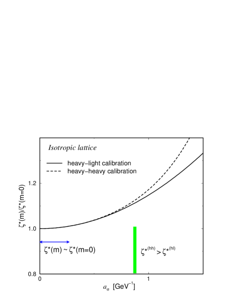
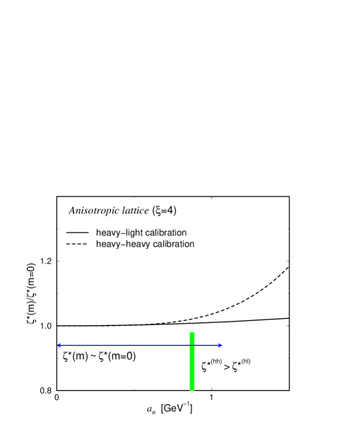
Figure 1: The conjecture of lattice spacing dependence of the anisotropy parameter for fixed quark mass, for isotropic (left) and anisotropic (right) lattices. Horizontal lines with arrows roughly represent the region $a_{\sigma}<a_{\sigma}^{hl\mbox{-}ll}$, while vertical thick lines correspond to $a_{\sigma}^{hh\mbox{-}hl}$, above which the $\zeta^{*}$’s determined from heavy-heavy and heavy-light mesons no longer equal. In this figure, a heavy quark with roughly the charm quark mass is considered as an example.

On an anisotropic lattice, one must tune the parameters so that the hadronic states satisfy the relativistic dispersion relations. In general, the lattice dispersion relation for arbitrary values of $\zeta$ is described in lattice units as

$$E^{2}(\mbox{\boldmath$p$})=m^{2}+\mbox{\boldmath$p$}^{2}/\xi_{F}^{2}+O(p^{4}).$$ (4)

In the above expression the energy $E$ and the rest mass $m$ are in temporal lattice units while the momentum $p$ is in spatial units. The parameter $\xi_{F}$ introduced in this equation characterizes the anisotropy of the quark fields. The difference between the quark field anisotropy $\xi_{F}$ and the gauge field anisotropy $\xi$ probes the breaking of relativity. Therefore, the calibration is nothing but the tuning of $\zeta(=1/\gamma_{F})$ for a given $\kappa$ so that $\xi_{F}$ equals $\xi$ and hence the relativistic dispersion relations are satisfied. Let us call the tuned parameter as $\zeta^{*}(=1/\gamma_{F}^{*})$. $\zeta^{*}$ depends on the quark mass and can in general be different from unity even for the case of isotropic lattice. The requirement of the relativity relation automatically enforces that the rest and kinetic masses are equal to each other. In this sense, our calibration procedure of anisotropic lattice action is a natural generalization of the Fermilab approach.

Now we consider the tuning of anisotropic parameter either on isotropic or anisotropic lattice, for fixed physical quark mass. The anisotropy parameter $\zeta=1/\gamma_{F}$ can be tuned using the dispersion relation of either heavy-heavy or heavy-light meson in mass dependent way. Alternatively, one can also adopt the value tuned for the light-light mesons neglecting the mass dependence. These procedures of calibration can give different results due to the discretization errors. We would like to know: 1) the value of lattice spacing $a_{\sigma}^{hh\mbox{-}hl}$ above which the calibrated parameters $\zeta^{*}$ using the heavy-heavy and heavy-light mesons differ from each other by more than a certain accuracy $\epsilon_{acc}$ (say, 2%), and 2) the value of lattice spacing $a_{\sigma}^{hl\mbox{-}ll}$ above which the calibrated parameters $\zeta^{*}$ using the heavy-light and light-light mesons are different by more than a certain accuracy $\epsilon^{\prime}_{acc}$.

Naively speaking, the difference between $\zeta^{*}$’s with heavy-heavy and heavy-light mesons originates from the $O((a_{\sigma}p)^{2})$ effects, where $p$ is the typical quark momenta in heavy-heavy meson, $p\sim\alpha m_{Q}$. On the other hand, the deviation of $\zeta^{*}$ with heavy-light mesons from the $\zeta^{*}$ with light-light mesons is due to the $O((a_{\tau}m_{Q})^{2})=O((a_{\sigma}m_{Q}/\xi)^{2})$ effects. With the criteria that these errors stay within the required accuracies, we obtain

$$a_{\sigma}^{hh\mbox{-}hl} \sim \sqrt{\epsilon_{acc}}/(\alpha m_{Q}),$$

$$a_{\sigma}^{hl\mbox{-}ll} \sim \sqrt{\epsilon^{\prime}_{acc}}~{}\xi/m_{Q}.$$ (5)

Figure 1 conjectures the expected behavior of the tuned anisotropy parameter $\zeta^{*}$ for the isotropic ($\xi=1$) and anisotropic ($\xi=4$) lattices. The tuned anisotropy normalized by the value at massless limit is displayed for fixed physical quark mass, around charm quark mass, as an example. In the case of isotropic lattice, as shown in the left panel of Fig. 1, $a_{\sigma}^{hl\mbox{-}ll}<a_{\sigma}^{hh\mbox{-}hl}$ is expected to hold. In this case, for a sufficiently small lattice spacing $a_{\sigma}<a_{\sigma}^{hl\mbox{-}ll}$, both the heavy-heavy and heavy-light mesons can be successfully described by setting the anisotropy parameter to the value in the massless limit. For a coarser lattice spacing $a_{\sigma}^{hl\mbox{-}ll}<a_{\sigma}<a_{\sigma}^{hh\mbox{-}hl}$ , mass dependent tuning, namely the Fermilab approach, is necessary, but the description of both the heavy-heavy and heavy-light mesons still works. For an even coarser lattice spacing $a_{\sigma}^{hh\mbox{-}hl}<a_{\sigma}$, simultaneously consistent description of heavy-heavy and heavy-light mesons no longer works, because of severe discretization effect in the heavy quarkonia.

Now let us consider the anisotropic lattice case with $\xi=4$. The expected mass dependence of $\zeta^{*}$ is schematically represented in the right panel of Fig. 1. As is obvious in Eq. (5) and will be studied in the following sections, the anisotropy does not improve the situation for heavy-heavy meson. Therefore $a_{\sigma}^{hh\mbox{-}hl}$ remains roughly of the same size as in the isotropic lattice case. On the other hand, Eq. (5) and the studies in the following sections show that for $\xi=4$, $a_{\sigma}^{hl\mbox{-}ll}$ is expected to increase and $a_{\sigma}^{hh\mbox{-}hl}<a_{\sigma}^{hl\mbox{-}ll}$ occasionally holds. This latter situation is particularly probable for quark with not very large mass, and expected to hold up to the bottom quark mass region. In this case, for sufficiently small lattice spacing $a_{\sigma}<a_{\sigma}^{hh\mbox{-}hl}$, both the heavy-heavy and heavy-light mesons can be successfully described by setting the anisotropy parameter to the value in the massless limit. For a coarser lattice spacing $a_{\sigma}^{hh\mbox{-}hl}<a_{\sigma}<a_{\sigma}^{hl\mbox{-}ll}$ consistent description of heavy-heavy and heavy-light mesons no longer works. Nevertheless the heavy-light meson is successfully described with the anisotropy parameter tuned for the massless limit. Finally for an even coarser lattice spacing $a_{\sigma}^{hl\mbox{-}ll}<a_{\sigma}$, the genuine Fermilab approach, namely mass dependent tuning of $\zeta$, is required to describe the heavy-light mesons.

In the range of lattice spacing $a_{\sigma}<a_{\sigma}^{hl\mbox{-}ll}$, if we give up the description of heavy quarkonia and only consider the heavy-light systems, one can successfully adopt the tuned value of $\zeta$ at the massless limit. This is the most important region for our approach, since there the mass dependence of parameters in the action other than $\zeta=1/\gamma_{F}$, such as $c_{E}$ and $c_{B}$, are also expected to be small, and hence the result of tuning at the massless limit is also considered to be valid. For the tuning of clover coefficient for the massless quark, it may be possible to apply the nonperturbative renormalization technique NRimp , which is currently most efficient procedure to remove the $O(a)$ effect beyond perturbation theory. The most advantage of the anisotropic lattice is that this region $a<a_{\sigma}^{hl\mbox{-}ll}$ is expected to be extended by a factor $\xi$ as is found in Eq. (5), so as to cover the heavy quark mass region of practical interests. Therefore the anisotropic lattice is a candidate of framework for heavy-light systems, which satisfies the required characters (i), (ii), and (iii) mentioned in the Introduction. Also for heavy-heavy systems, it would be important to study quantitatively the heavy quark mass at which the action starts to fail in correct description.

This paper is dedicated to a numerical study whether these expectations actually holds. Using Eq. (5), similar expectation can be deduced for the heavy quark mass dependence with a fixed lattice spacing. In this paper, since we work with only one lattice spacing, instead of studying the lattice spacing dependence with a fixed heavy quark mass, we study the mass dependence with a fixed lattice spacing. This means to specify in which region considered above the present $a_{\sigma}$ is located for each value of quark mass. This subject is discussed in more detail with the tree level analysis in the next section, and with the numerical simulation in the successive section.

III Expectation from tree level analysis

In this section, we review the tree level analysis of the heavy quark action in the Fermilab formulation. In the following, we express the energy and the momenta in physical units so that the dependence on the lattice spacings $a_{\tau}$ and $a_{\sigma}$ is explicitly shown. The dispersion relation of the heavy quark on anisotropic lattice is given as EKM97 ; Aniso01a

$$\cosh(a_{\tau}E) = 1+$$ (6)

$$\frac{[\overline{m}_{0}+2r\zeta\sum_{i}\sin^{2}(a_{\sigma}p_{i}/2)]^{2}+\zeta^{2}\sum_{i}\sin^{2}(a_{\sigma}p_{i})}{2[1+\overline{m}_{0}+2r\zeta\sum_{i}\sin^{2}(a_{\sigma}p_{i}/2)]},$$

where $\overline{m}_{0}=a_{\tau}m_{0}$ . This leads to the following dispersion relation.

$$E^{2} = M_{1}^{2}+\left(\frac{\xi^{\rm tree}}{\xi_{F}^{\rm tree}}\right)^{2}\mbox{\boldmath$p$}^{2}$$ (7)

$$+A_{1}a_{\sigma}^{2}(\mbox{\boldmath$p$}^{2})^{2}+A_{2}a_{\sigma}^{2}\sum_{i}p_{i}^{4}+\cdots,$$

where $M_{1}$ is the pole mass,

$$M_{1} = \log(1+\overline{m}_{0})a_{\tau}^{-1},$$ (8)

and the anisotropy of the quark field at the tree level,

$$\left(\frac{\xi^{\rm tree}}{\xi_{F}^{\rm tree}}\right)^{2}=\log(1+\overline{m}_{0})\xi^{2}\left[\frac{2\zeta^{2}}{\overline{m}_{0}(2+\overline{m}_{0})}+\frac{r\zeta}{1+\overline{m}_{0}}\right].$$ (9)

The third and fourth terms in Eq (7) represent the $O((ap)^{2})$ errors, where $A_{1}$ and $A_{2}$ are given as

$$A_{1} = \frac{\xi^{2}}{4}\left[\left(\frac{2\zeta^{2}}{\overline{m}_{0}(2+\overline{m}_{0})}+\frac{r\zeta}{1+\overline{m}_{0}}\right)^{2}\right.$$ (10)

$$-\log(1+\overline{m}_{0})\left(\frac{8\zeta^{4}}{\overline{m}_{0}^{3}(2+\overline{m}_{0})^{3}}\right.$$

$$\left.\left.+\frac{4\zeta^{3}[\zeta+2r(1+\overline{m}_{0})]}{\overline{m}_{0}^{2}(2+\overline{m}_{0})^{2}}+\frac{r^{2}\zeta^{2}}{(1+\overline{m}_{0})^{2}}\right)\right],$$

$$A_{2}=-\frac{\xi^{2}}{3}\log(1+\overline{m}_{0})\left[\frac{2\zeta^{2}}{\overline{m}_{0}(2+\overline{m}_{0})}+\frac{r\zeta}{4(1+\overline{m}_{0})}\right].$$ (11)

The above coefficients are derived using the $M_{1}$, $M_{2}$, $M_{4}$ and $w_{4}$ in Ref. EKM97 extended to anisotropic lattice by replacing certain parameters as given in Ref. Aniso01a .

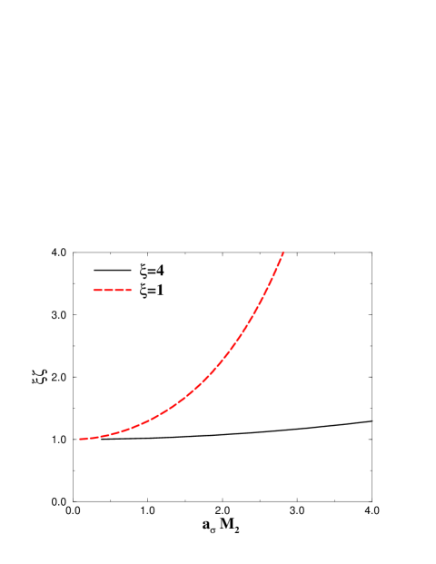
Figure 2: The mass dependence of $\xi\zeta$ tuned at the tree level for the isotropic lattice and anisotropic lattice with $\xi=4$. The horizontal axis is the kinetic quark mass in spatial lattice units.

Fig. 2 shows the mass dependence of $\zeta$ tuned by requiring $\xi_{F}=\xi$, both on the isotropic lattice and on the anisotropic lattice with $\xi=4$. In the latter case, it is clear that the mass dependence is drastically reduced so that taking the value of $\zeta$ with massless limit is a good approximation over a wide range of quark mass, in contrast to the case of the isotropic lattice.

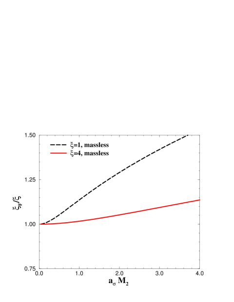
Figure 3: The kinetic mass dependence of $\xi_{F}/\xi$ at the tree level. We do not show the the result of mass dependent tuning of $\zeta$ since $\xi_{F}/\xi=1$ is satisfied by definition.

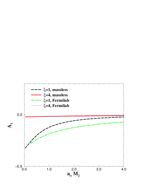
Figure 4: The kinetic mass dependence of the $O((ap)^{2})$ coefficient $A_{1}$ in the dispersion relation (7). “massless ” denotes the result of tuning of $\zeta$ in the massless limit. “Fermilab” denotes the result of mass dependent tuning of $\zeta$ by requiring $\xi_{F}=\xi$.

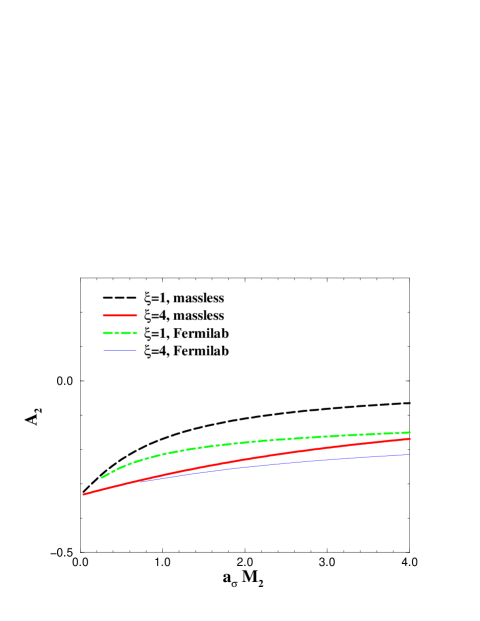
Figure 5: The kinetic mass dependence of the $O((ap)^{2})$ coefficient $A_{2}$ in the dispersion relation (7).

In the following, let us consider either the case with mass dependent tuning of $\zeta$ (denoted by “Fermilab” in the figures) or with the $\zeta$ at the massless limit (“massless”). Figure 3 shows the breaking effect of relativity relation, $\xi_{F}/\xi$, according to Eq. (9). The kinetic mass $M_{2}$ of quark is related to $\xi_{F}/\xi$ as $M_{2}=M_{1}\xi_{F}^{2}/\xi^{2}$. For the mass dependently tuned $\zeta$, $\xi_{F}$ trivially equals $\xi$. Without tuning, the mass dependence of $\xi_{F}$ is drastically reduced in the case of $\xi=4$, as is expected from that the deviation of $\xi_{F}/\xi$ from unity is the $O(a_{\tau}m_{Q})$ error. In Figure 4, one find that the coefficient $A_{1}$, whose deviation from zero signals the $O(a^{2})$ effect, is also drastically reduced on the anisotropic lattice, either with or without mass dependent tuning of $\zeta$. On the other hand, $O(a^{2})$ error from $A_{2}$ is not reduced but somewhat worse on the anisotropic lattice as is seen in Figure 5. However, the coefficient $A_{2}$ is not larger than the value at the massless limit. As a general feature for all of the $\xi_{F}/\xi$, $A_{1}$ and $A_{2}$, the mass dependences are drastically reduced on the anisotropic lattice. On the other hand, mass dependent tuning of $\zeta$ on isotropic lattice does not reduce the coefficients $A_{1}$ and $A_{2}$, while it completely removes the discrepancy between $\xi_{F}$ and $\xi$. In order to reduce these errors one has to introduce higher order terms as is pointed out in Ref.  EKM97 .

From these results, one can expect the following about the error of the heavy quark systems. For the heavy-light systems, since heavy quark momenta typically takes the size of the hadronic scale, $\Lambda_{QCD}\simeq$ 200–500 MeV, the $O((ap)^{2})$ errors are well under control even for large $a_{\sigma}M_{2}$, if one keep $a_{\sigma}^{-1}\gg\Lambda_{QCD}$. While the largest error originates from $A_{2}$, this is of the same order as that in the light quark systems. For the heavy-heavy system, the situation is quite different. Since the heavy quark momenta are typically $p\sim\alpha m_{Q}$, The $O((ap)^{2})$ errors are expected to be as large as $A_{1}(\alpha a_{\sigma}m_{Q})^{2}$, $A_{2}(\alpha a_{\sigma}m_{Q})^{2}$. Again the $A_{2}$ gives the largest contribution, but the size of the error is uncontrolled when $a_{\sigma}m_{Q}$ is large.

To summarize, the anisotropic lattice largely reduces the discretization effects represented by $\xi_{F}/\xi-1$ and $A_{1}$, while it does not improve the $A_{2}$. For the heavy-light systems, this suffices for a computation with discretization effects under control. On the other hand, when $a_{\sigma}M_{2}$ is of order of unity, the anisotropic lattice does not improve the situation for heavy quarkonia, because of severe effect of $A_{2}$ in these systems. Although mass dependent tuning of $\zeta$ further removes the deviation of $\xi_{F}$ from $\xi$, the $\zeta$ tuned for massless quark also stay a good approximation if $a_{\tau}m_{0}\ll 1$ holds. This is the most advantage of anisotropic lattice compared with the isotropic Fermilab approach, in which the mass dependence of the parameter is much stronger. These observations are in accord with our conjecture in the last section for developing the anisotropic Fermilab formulation.

IV Numerical simulation

This section numerically examines the idea described in previous sections. For this purpose, we perform simulations with two series of heavy quark parameters. For Set-I the anisotropy parameter is set to the value at the chiral limit, $\gamma_{F}^{*}(m_{q}=0)$, just as same as for the light quark. The Set-II adopts the fully tuned anisotropy parameter $\gamma_{F}^{*}$ using heavy-heavy mesons. This calibration is done in the first subsection. For the heavy-heavy and heavy-light mesons, the rest and kinetic masses are obtained with two sets of parameters. Two quantities are used to probe the breaking effect of the relativity: the fermionic anisotropy $\xi_{F}$ for heavy-heavy and heavy-light mesons, and the inconsistency among the binding energies of heavy-heavy, heavy-light, and light-light mesons. These behaviors give us a hint to judge the regions in which our framework can be applied. The last subsection treats the heavy-light meson spectrum, and observe how the hyperfine splitting behaves with meson kinetic mass.

IV.1 Calibration in heavy quark region

The simulation parameters used in this paper is the second set in Ref. Aniso01b : the quenched anisotropic lattice of the size $16^{3}\times 128$ generated with the standard plaquette gauge action with $(\beta,\gamma_{G})=(5.95,3.1586)$, which correspond to the renormalized anisotropy $\xi=4$ Kla98b and spatial lattice cutoff $a_{\sigma}^{-1}=1.623(9)$ GeV set by hadronic radius $r_{0}$ Som94 . The mean-field values in the quark action are set to the mean values of link variables in the Landau gauge: $u_{\sigma}=0.7917$ and $u_{\tau}=0.9891$.

In Ref. Aniso01b , the optimum bare anisotropy $\gamma_{F}^{*}$ is determined using the dispersion relation of mesons with degenerate quark masses, and the resultant values of $\gamma_{F}^{*}$ are well represented by a linear function

$$\frac{1}{\gamma_{F}^{*}}=\zeta_{0}+\zeta_{2}m_{q}^{2},\hskip 19.91684ptm_{q}=\frac{1}{2\xi}\left(\frac{1}{\kappa}-\frac{1}{\kappa_{c}}\right),$$ (12)

where for the present lattice $\zeta_{0}=0.2490(8)$, $\zeta_{2}=0.189(15)$, and $\kappa_{c}=0.12592(6)$.

Table 1: Quark parameters and the result of calibration. The result for $\kappa=0.1100$, $0.1020$, and $0.0930$ are taken from Ref. Aniso01b . The number of configurations is 200 for each value of the hopping parameter, except for $\kappa=0.1100$ for which the simulation is carried out with 300 configurations.

$\kappa$	$m_{0}$	input $\gamma_{F}$	$\gamma_{F}^{*(PS)}$	$\gamma_{F}^{*(V)}$	$\gamma_{F}^{*}$	$\delta\gamma_{F}^{*}$
0.1100	0.1437	3.90, 4.00	3.945(28)	3.946(36)	3.946(29)	-0.001(20)
0.1020	0.2328	3.90, 4.00	3.848(26)	3.847(34)	3.847(28)	0.001(15)
0.0930	0.3514	3.70, 3.80	3.688(23)	3.687(29)	3.688(25)	0.000(11)
0.0840	0.4954	3.39, 3.48	3.471(20)	3.462(23)	3.467(21)	0.0092(60)
0.0760	0.6521	3.04, 3.15	3.205(20)	3.191(23)	3.199(21)	0.0139(45)
0.0700	0.7930	2.85, 2.95	2.946(23)	2.932(23)	2.939(23)	0.0134(52)
0.0630	0.9914	2.50, 2,60	2.584(22)	2.561(24)	2.573(23)	0.0237(35)

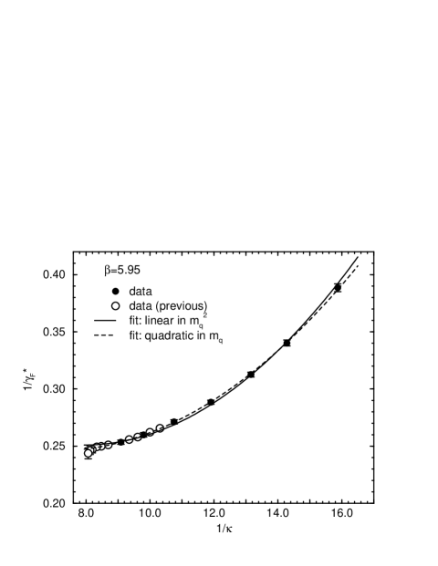
Figure 6: The result of calibration in the heavy quark mass region (filled circles), together with the previous result in Ref. Aniso01b . The fits are performed with all available data including previous results.

In this paper, we use seven values of $\kappa$ for heavy quark ($\kappa_{h}$), which roughly cover 1–6 GeV. Three of them already appeared in Ref. Aniso01b . We start with the calibration of remaining four values of $\kappa$ in the heavy quark region in the same manner as in Ref. Aniso01b . The values of $\kappa$ used are listed in Table 1 together with the result of calibration. The second column is the naive estimate of bare quark mass according to Eq. (12). For the heaviest case, $m_{0}$ is almost unity in temporal lattice units, and therefore the breaking effect of relativity may be visible. Here we note that for heavier quark masses the difference of $\gamma_{F}^{*}$ for pseudoscalar and vector mesons,

$$\delta\gamma_{F}^{*}=\gamma_{F}^{*(V)}-\gamma_{F}^{*(PS)},$$ (13)

is sizable beyond the statistical fluctuations. This signals that the quarkonium system is not properly described within the present framework at this lattice spacing. This problem will again be discussed later in terms of the fermionic anisotropies for heavy-heavy and heavy-light mesons.

Figure 6 shows the result of calibration. The result is well fitted to a linear form in $m_{q}^{2}$ or a quadratic form in $m_{q}$, in spite of large quark mass. The fits including previous data in Ref. Aniso01b result in

Linear: $$\zeta_{0}=0.2510(6),\ \zeta_{2}=0.1437(26).$$ (14)

Quadratic: $$\zeta_{0}=0.2473(12),\ \zeta_{1}=0.0267(72),$$ (15)

$$\hskip 28.45274pt\zeta_{2}=0.1151(81).$$

In both cases, the values of $\zeta_{0}$ is close to the value at the mean-field tree level, $\xi^{-1}=0.25$. Since there is no reason that the small quark mass dependence persist up to $m_{q}\simeq a_{\tau}^{-1}$, the difference between $\zeta_{2}$’s in linear fits with present data and with only previous data in lighter quark mass region is irrelevant, and above result just shows that the quark mass dependence of $1/\gamma_{F}^{*}$ is still tractable at this mass region.

IV.2 Relativity breaking effect

In this subsection we compute the heavy-heavy and heavy-light meson spectra and the dispersion relations using two sets of heavy quark parameters. For the first one, Set-I, the bare anisotropy is set to the value of $\gamma_{F}^{*}$ in the chiral limit obtained in Ref. Aniso01b , namely $\gamma_{F}=4.016$ at $\beta=5.95$, for all quark masses. The second one, Set-II, adopts the above result of mass dependent calibration. We use the same hopping parameter values $\kappa_{h}$ for the heavy quark as given in the previous subsection. For the light quark, we use single value, $\kappa_{l}=0.1235$. The value of $\gamma_{F}$ at this $\kappa_{l}$ is set to the value in the chiral limit, as same as in the light hadron spectroscopy in Ref. Aniso01b . We regard that at $\kappa=\kappa_{l}$ the quark mass is sufficiently light for present purposes, and do not extrapolate to the chiral limit. The numbers of configurations used are 200 and 500 for heavy-heavy and heavy-light meson masses, respectively.

Table 2: Heavy-heavy meson spectrum for Set-I and Set-II parameters obtained with 200 configurations.

	$\kappa_{h}$	$\gamma_{F}$	$m_{PS}$	$m_{V}$	$m_{V}-m_{PS}$	$\xi_{F}^{(PS)}$	$\xi_{F}^{(V)}$	$\xi_{F}^{(V)}-\xi_{F}^{(PS)}$
Set-I	0.1100	4.016	0.42468(23)	0.43755(33)	0.01288(18)	4.069(34)	4.068(46)	-0.001(24)
	0.1020	4.016	0.58409(25)	0.59358(34)	0.00949(13)	4.148(27)	4.143(35)	-0.005(16)
	0.0930	4.016	0.76947(24)	0.77692(31)	0.00745(10)	4.292(22)	4.294(28)	0.002(10)
	0.0840	4.016	0.96746(25)	0.97358(31)	0.00612( 8)	4.527(24)	4.537(29)	0.010( 8)
	0.0760	4.016	1.15894(27)	1.16411(33)	0.00517( 8)	4.821(30)	4.839(35)	0.018(10)
	0.0700	4.016	1.31453(27)	1.31896(31)	0.00443( 7)	5.146(33)	5.187(38)	0.041( 8)
	0.0630	4.016	1.51262(27)	1.51617(31)	0.00355( 5)	5.650(39)	5.726(43)	0.076( 7)
Set-II	0.1100	3.946	0.42942(23)	0.44248(33)	0.01306(18)	4.005(29)	4.003(41)	-0.002(22)
	0.1020	3.847	0.60172(25)	0.61146(33)	0.00975(14)	4.002(24)	4.000(32)	-0.003(14)
	0.0930	3.688	0.81797(24)	0.82574(31)	0.00777(10)	3.995(19)	4.000(24)	0.005( 9)
	0.0840	3.467	1.07512(25)	1.08167(30)	0.00655( 7)	3.996(18)	4.005(22)	0.009( 6)
	0.0760	3.199	1.35939(26)	1.36509(31)	0.00571( 7)	4.002(22)	4.011(26)	0.010( 6)
	0.0700	2.939	1.62650(27)	1.63164(31)	0.00514( 6)	3.993(23)	4.009(26)	0.016( 5)
	0.0630	2.573	2.02101(28)	2.02550(31)	0.00449( 5)	3.988(23)	4.013(26)	0.025( 4)

Table 3: Heavy-light meson spectrum for Set-I and Set-II parameters obtained with 500 configurations.

	$\kappa_{h}$	$m_{PS}$	$m_{V}$	$m_{V}-m_{PS}$	$\xi_{F}^{(PS)}$	$\xi_{F}^{(V)}$	$\xi_{F}^{(V)}-\xi_{F}^{(PS)}$
Set-I	0.1100	0.29108(27)	0.30997(51)	0.01889(39)	3.985(36)	4.006(49)	0.020(44)
	0.1020	0.37705(30)	0.39106(50)	0.01401(34)	3.994(39)	4.031(51)	0.036(42)
	0.0930	0.47595(36)	0.48643(57)	0.01048(36)	4.032(51)	4.101(73)	0.070(55)
	0.0840	0.58123(46)	0.58123(46)	0.00805(43)	4.088(73)	4.21(11)	0.119(77)
	0.0760	0.68279(55)	0.68916(81)	0.00638(44)	4.148(99)	4.30(15)	0.147(87)
	0.0700	0.76546(64)	0.77079(89)	0.00534(45)	4.21(13)	4.38(18)	0.173(98)
	0.0630	0.87080(78)	0.8751(10)	0.00430(47)	4.30(18)	4.51(25)	0.21(12)
Set-II	0.1100	0.29323(27)	0.31229(52)	0.01906(39)	3.952(36)	3.970(48)	0.018(44)
	0.1020	0.38526(30)	0.39961(50)	0.01435(34)	3.905(37)	3.936(49)	0.031(40)
	0.0930	0.49889(35)	0.50990(57)	0.01101(37)	3.846(46)	3.904(66)	0.058(51)
	0.0840	0.63258(40)	0.64135(60)	0.00877(36)	3.757(54)	3.829(76)	0.071(54)
	0.0760	0.77918(49)	0.78647(75)	0.00729(43)	3.666(73)	3.77(11)	0.108(71)
	0.0700	0.91609(54)	0.92246(80)	0.00637(44)	3.571(84)	3.69(12)	0.118(73)
	0.0630	1.11749(62)	1.12294(87)	0.00544(45)	3.45(10)	3.58(14)	0.130(77)

The meson spectra are listed in Table 2 and 3 for heavy-heavy and heavy-light mesons, respectively. In these tables, we also list the results of $\xi_{F}$ for each meson channel, and difference between them, $\delta\xi_{F}=\xi_{F}^{(V)}-\xi_{F}^{(PS)}$. If the anisotropic lattice action does not describe the quarks inside mesons in respecting the relativity relation, the breaking effect appears in the dispersion relations of mesons. Therefore the deviation of fermionic anisotropy $\xi_{F}$ from $\xi$ signals the breaking effect of relativity. In the following, we first discuss on the result of $\xi_{F}$ for Set-I parameters, namely with $\gamma_{F}$ tuned for massless limit, and then briefly summarize the result for Set-II parameters.

Figure 7 displays the heavy quark mass dependence of $\xi_{F}$ for Set-I. The horizontal axis is the bare quark mass $m_{q}$ in temporal lattice units. The behaviors of $\xi_{F}$’s are well in accord with the expectation in Sec. II. For quantitative discussion, let us consider the case that the required accuracies to define the $a_{\sigma}^{hh\mbox{-}hl}$ and $a_{\sigma}^{hl\mbox{-}ll}$ are 2 %, namely $\epsilon_{acc}=\epsilon_{acc}=0.02$. $\xi_{F}$’s from the heavy-heavy and heavy-light mesons disagree beyond this accuracy at $m_{q}>0.2$ ($a_{\sigma}m_{Q}>0.8$). Therefore one must keep $m_{q}<0.2$ to avoid large systematic uncertainty in the heavy quarkonia. On the other hand, the $\xi_{F}$ from the heavy-light mesons are rather close to $\xi$, and $\gamma_{F}^{*}(m_{q}=0)$ can be applied up to $m_{q}\simeq 0.3$ within presently required accuracy. For quark mass larger than this value, the discrepancy between $\xi_{F}$’s from the pseudoscalar and vector mesons gradually grows beyond the statistical error. This signals the growth of systematic error. In the region of $m_{q}<0.3$ such effect is sufficiently small.

For the charm quark mass, the present lattice spacing $a_{\sigma}$ is already well less than $a_{\sigma}^{hl\mbox{-}ll}$ so that the $\gamma_{F}$ tuned for massless quark is applicable to the charmed hadron systems. On the other hand, bottom quark mass is not the case, and one need finer lattice spacing or larger anisotropy $\xi$. The present lattice would be also sufficient for the charmonium states, since the region $m_{q}<0.2$ also covers the charm quark mass. Another striking feature is that the observed $\xi_{F}$’s for heavy-light mesons are close to the tree level expectation. This implies that the deviation of $\xi_{F}$ from $\xi$ may be largely removed by the tree level tuning of $\gamma_{F}$. Such an approach would work for the spectroscopy of hadrons containing single bottom quark. This is a good alternative procedure to the mass dependent calibration using heavy-light meson, since the statistical error of $\xi_{F}$ from heavy-light mesons rapidly grows as heavy quark mass.

Now we summarize the result for the Set-II. The heavy-heavy meson satisfies the relativity relation by definition. However, the heavy-light meson dispersion relation violates the relativity relation so that $\xi_{F}/\xi$ deviates from unity toward smaller value as heavy quark mass increases. This implies that the mass dependent tuning cannot absorb the discrepancy between the $\xi_{F}$’s from the heavy-heavy and heavy-light meson systems. For the quark mass of $m_{q}<0.2$, the result for Set-II are consistent with the result for Set-I. In that region the heavy-heavy meson can be successfully described, and therefore the result of calibration with heavy-heavy mesons is also valid.

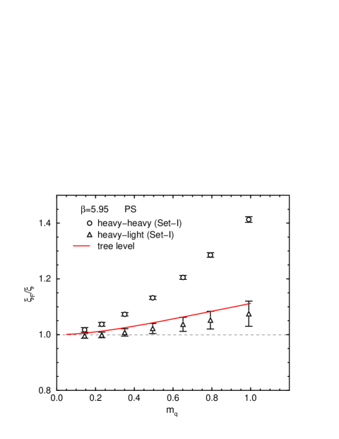
Figure 7: Fermionic anisotropy determined nonperturbatively from the dispersion relations of heavy-heavy and heavy-light mesons. The left and right panels show the results for the pseudoscalar and vector channels, respectively. The solid lines represent the tree level values according to Eq. (9).

We now observe the inconsistency among the binding energies of heavy-heavy, heavy-light, and light-light mesons discussed in Refs. SAnomaly1 ; SAnomaly2 . The inconsistency is probed by a quantity

$$I\equiv\frac{2\delta M_{hl}-(\delta M_{hh}+\delta M_{ll})}{2M_{2hl}},$$ (16)

where $\delta M=M_{2}-M_{1}$, $M_{1}$ and $M_{2}$ are the rest and kinetic masses of the meson, respectively. The subscripts $hh$, $hl$, and $ll$ represent the quark contents of each meson ($h$ for heavy and $l$ light quarks). We neglect the last term in the numerator, since the calibration of light quark mass region requires that $\delta M_{ll}$ vanishes. Since the rest and kinetic quark masses cancel in each kind of mass, nonvanishing $I$ represents the inconsistency in the binding energy, namely the dynamical effect. The anomalous behavior of $I$ in large kinetic mass region was first reported in Ref. SAnomaly1 for the $O(a)$ improved quark action on isotropic lattice. Ref. SAnomaly2 explained that this behavior originates from the $O((ap)^{2})$ discretization effect in the heavy quarkonium system and estimate the size of $I$ with the help of potential model analysis. It results in $I\simeq-0.5$ at $aM_{2hl}\simeq 3.2$, which is in good agreement with the result in SAnomaly1 .

Figure 8 displays the results of $I$ for Set-I and II for the pseudoscalar channel. The behavior of $I$ is quite similar to that in Refs. SAnomaly1 ; SAnomaly2 , as is expected from that it originates from $O((a_{\sigma}p)^{2})$ error and therefore is not improved by the anisotropy. The behavior of $I$ of two sets is very similar to each other. It means that the inconsistency cannot be eliminated by tuning anisotropy parameters with either heavy-heavy or heavy-light system, and a kind of universal quantity to signal the failure in consistent description of heavy quarkonium systems. The $I$ rapidly deviate from zero for the heavy quark mass larger than our lightest one. This is consistent with the above observation of $\xi_{F}$.

These results indicate that for $a_{\tau}m_{Q}>0.2$ the present action fails to describe the dynamics of heavy quarkonium, and cannot be reinterpreted by the subtraction of quark mass effect. Thus we need to either give up to apply the present framework for such a quark mass region, or to improve the action by incorporating higher order correction terms. The remaining part of this section therefore focus on the heavy-light meson spectrum.

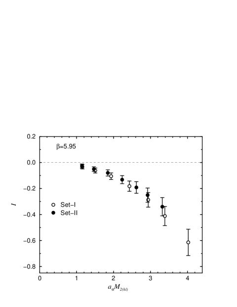
Figure 8: The inconsistency among the binding energies of heavy-heavy, heavy-light and light-light mesons. The horizontal axis is in spatial lattice units.

IV.3 Heavy-light meson spectrum

Now we turn our attention to the heavy-light meson, which is of our main interest. According to the heavy quark expansion, the spin flipping interaction of heavy quark in the heavy-light systems is of $O(1/m_{Q})$, and hence the hyperfine splitting of mesons is proportional to the meson mass at the leading order. In the heavy-light systems, the large mass of heavy quark is not important for the dynamics. Employing the Fermilab formulation, this character is taken into account and the the correct heavy quark expansion is in terms of kinetic mass EKM97 . Therefore, the hyperfine splitting, which is measured as the difference of rest masses, are expected to be reciprocally proportional to the kinetic meson mass. If this is the case, Set-I and Set-II should show the similar behaviors, up to the $O(a^{2})$ systematic uncertainty.

The hyperfine splitting $m_{V}-m_{PS}$ is displayed in Figure 9. The horizontal axis is spin averaged kinetic meson mass inverse in physical units defined through the hadronic radius $r_{0}$. Since the most serious uncertainty in the kinetic mass is from the systematic uncertainty in $\xi_{F}$, we estimate this error as

$$\delta M_{2}=2M_{2}|\delta\xi_{F}|/\xi_{F},$$ (17)

where $\delta\xi_{F}=\xi_{F}^{(V)}-\xi_{F}^{(PS)}$, and hence it does not include the statistical errors of $\xi_{F}$ and $M_{2}$. On the other hand, the error associated to the hyperfine splitting is the statistical one. Although the data shows a linear dependence in the heavy quark mass region, there appears small negative intercept. We regard this small discrepancy with the heavy quark expansion as the Lorentz symmetry breaking effect brought in the meson dispersion relation and of $O(a^{2})$. For fixed physical quark mass, this effect is expected to disappear linearly in $a^{2}$ toward the continuum limit. The results of Set-I and Set-II clearly show similar behavior, and therefore the above interpretation of Fermilab formulation works well up to the relativity breaking effect represented by $\delta\xi_{F}$. For more quantitative analysis, one must quantify the size of $O(a^{2})$ systematic errors and observe how they disappear toward the continuum limit. This is out of the scope of this paper.

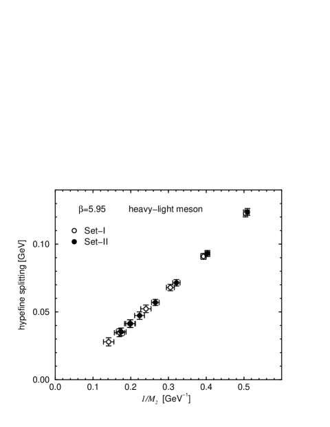
Figure 9: The hyperfine splitting of heavy-light meson versus the inverse of the heavy-light meson kinetic mass. The physical scale is set by the hadronic radius $r_{0}$. The error in $1/M_{2}$ is the systematic one estimated from the discrepancy of $\xi_{F}$ from pseudoscalar and vector mesons.

V Conclusion

In this paper, we investigated an applicability of the anisotropic lattice quark action in heavy quark mass region, on the quenched lattice with $a_{\sigma}^{-1}\simeq 1.6$ GeV and renormalized anisotropy $\xi=4$. The anisotropy is expected to extend the region in which the parameters in the action tuned for massless quark are applicable to precision computations of heavy-light matrix elements. For this purpose, we measured the heavy-heavy and heavy-light meson masses and dispersion relations to observe the relativity breaking effect. The calculation was carried out for two sets of parameters, Set-I and Set-II. Set-I adopts the values at the massless limit, while in Set-II the bare anisotropy is tuned using the heavy-heavy mesons. Our main results are as follows.

(a) In the quark mass region $a_{\tau}m_{Q}<0.2$, the observed fermionic anisotropy $\xi_{F}$’s are consistent for heavy-heavy and heavy-light mesons as well as for Set-I and Set-II parameters within 2 % accuracy. This implies that present framework is applicable to both these systems even without tuning of anisotropy parameter. Beyond this region, the action fails to describe the heavy quarkonium state correctly, as expected from the tree level analysis of the quark dispersion relation.

(b) The mass dependence of the renormalized anisotropy for the heavy-light mesons with $\gamma_{F}^{*}$ at the massless limit (Set-I) is so small that one can exploit the massless tuning in the region of $a_{\tau}m_{Q}<0.3$ with less than 2% errors. This result is essentially important for our strategy, since it implies that the parameters tuned at the massless limit is directly available for this mass region, which already contains charm quark mass with the present lattice and can be extended to the bottom quark with development of computational resources in successive decade.

(c) For $a_{\tau}m_{Q}>0.3$, relativity breaking effect in the heavy-light mesons seems to grow as a function of the heavy quark mass. This is signaled by the discrepancy of $\xi_{F}$’s from the pseudoscalar and vector mesons, although the present statistics is not enough for a quantitative estimate of this effect. In the scaling of hyperfine splitting, we also found small discrepancy with the expectation from the heavy quark expansion, which is considered as $O(a^{2})$ systematic effect. It is important to quantify these effects and to observe how they disappear toward the continuum limit, for future high precision computations with this approach.

We therefore conclude that the anisotropic lattice quark action satisfies the required characters (i)–(iii) for high precision calculations of heavy-light matrix elements mentioned in Introduction. Among above results, the small mass dependence of anisotropy parameter is in particular quite encouraging for further development of the framework in this direction.

One of the promising strategies is to calibrate the parameters in the action at the massless limit and use them for all masses. This should work perfectly for $a_{\tau}m_{Q}<0.3$ which is already sufficient to describe the $D$ meson systems. If one wants to treat $B$ meson systems, one has to work with heavier quark, $a_{\tau}m_{Q}>0.3$, in which case the mass dependent errors cannot be neglected. However, since the mass dependence is small, it can be interpreted as an $O(a^{2})$ error and can be removed by taking the continuum limit. Alternatively, one can also apply the genuine Fermilab approach for the bottom quark. In this case, the mass dependences of the renormalization coefficients are the source of systematic errors. Nevertheless, as long as one obtains such coefficients nonperturbatively in the massless limit first, and use the one-loop perturbation theory only to compute the mass dependent corrections, the perturbative error can be much better controlled compared to the Fermilab approach on the isotropic lattice. The nice agreement between the observed $\xi_{F}$ and the tree level expectation suggest that this idea is also promising in the bottom quark mass region.

On the other hand, present level of systematic errors as well as the statistical one is not sufficient for these ends. As a most significant example, one need to eliminate the $O(\alpha a)$ error using nonperturbative renormalization technique in the massless limit Kla98a , and confirm that this suffices also for heavy quark mass region treated in this paper.

References

- (1) For recent reviews, S. M. Ryan, Nucl. Phys. B (Proc. Suppl.) 106, 86 (2002); C. W. Bernard, Nucl. Phys. B (Proc. Suppl.) 94, 159 (2001).
- (2) For CLEO-c project, CLEO Collaboration, http://www.lns.cornell.edu/public/CLEO/.
- (3) For KEK B-factory experiment, Belle Collaboration, http://bsunsrv1.kek.jp/.
- (4) For SLAC B-factory experiment, BaBar Collaboration, http://www.slac.stanford.edu/BFROOT/.
- (5) B. A. Thacker and G. P. Lepage, Phys. Rev. D 43, 196 (1991).
- (6) M. Kurth and R. Sommer, (ALPHA Collaboration), Nucl. Phys. B623, 271 (2002).
- (7) A. X. El-Khadra, A. S. Kronfeld and P. B. Mackenzie, Phys. Rev. D 55, 3933 (1997).
- (8) Z. Sroczynski, A. X. El-Khadra, A. S. Kronfeld, P. B. Mackenzie and J. N. Simone, Nucl. Phys. B (Proc. Suppl.) 83, 971 (2000).
- (9) S. Aoki, Y. Kuramashi and S. Tominaga, hep-lat/0107009.
- (10) M. Lüscher, S. Sint, R. Sommer, P. Weisz and U. Wolff, Nucl. Phys. B491, 323 (1997).
- (11) T. R. Klassen, Nucl. Phys. B509, 391 (1998); Nucl. Phys. B (Proc. Suppl.) 73, 918 (1999).
- (12) J. Harada, A. S. Kronfeld, H. Matsufuru, N. Nakajima and T. Onogi, Phys. Rev. D 64, 074501 (2001).
- (13) H. Matsufuru, T. Onogi and T. Umeda, Phys. Rev. D 64, 114503 (2001).
- (14) S. Collins, R. G. Edwards, U. M. Heller, and J. Sloan, Nucl. Phys. B (Proc. Suppl.) 47, 455 (1996).
- (15) A. S. Kronfeld, Nucl. Phys. B (Proc. Suppl.) 53, 401 (1997).
- (16) T. Umeda, R. Katayama, O. Miyamura and H. Matsufuru, Int. J. Mod. Phys. A 16, 2215 (2001).
- (17) G. P. Lepage and P. B. Mackenzie, Phys. Rev. D 48, 2250 (1993).
- (18) T. R. Klassen, Nucl. Phys. B533, 557 (1998).
- (19) R. Sommer, Nucl. Phys. B411, 839 (1994).