MIT-CTP-3253

NON-PERTURBATIVE FORMULATION OF THE
STATIC COLOR OCTET POTENTIAL

Owe Philipsen

Center for Theoretical Physics,
Massachusetts Institute of Technology,
Cambridge, MA 02139-4307, USA

By dressing Polyakov lines with appropriate functionals of the gauge fields, we construct observables describing a fundamental representation static quark-antiquark pair in the singlet, adjoint and average channels of SU(N) pure gauge theory. Each of the potentials represents a gauge invariant eigenvalue of the Hamiltonian. Numerical simulations are performed for SU(2) in 2+1 dimensions. The adjoint channel is found to be repulsive at small and confining at large separations, suggesting the existence of a metastable $(N^{2}-1)$-plet bound state. For small distances and temperatures above the deconfinement transition, the leading order perturbative prediction for the ratio of singlet and adjoint potentials is reproduced by the lattice data.

The potential of two static color charges in the fundamental representation separated by a distance $r$ is a quantity of fundamental importance for the study of the confining force in SU(N) Yang-Mills theory and QCD, as well as the phenomenology of heavy quark systems. A quark-antiquark pair at the same point can be in either a singlet or an adjoint state, acccording to the irreducible representations of the tensor product

$$\bar{N}\otimes N=1+(N^{2}-1).$$ (1)

In perturbation theory, one fixes a gauge and a separate description for the two channels is possible also for small separations between the charges. To leading order one finds the relation (${\cal O}(g^{2})$ contributions cancel) [1, 2]

$$V_{1}(r)=-(N^{2}-1)V_{N^{2}-1}(r)+{\cal O}(g^{4}).$$ (2)

Because of the growing interaction strength, perturbation theory can be trusted only at short distances, while non-perturbative methods such as lattice simulations are required in the regime of linear confinement.

On the other hand, in lattice gauge theory one is interested in non-perturbatively gauge invariant quantities only. It has so far not been possible to construct such operators for the two channels separately. At zero temperature, the standard lattice operator to compute the static potential is the Wilson loop projecting onto the singlet channel. Good agreement between an integration of perturbatively truncated renomalization group equations and continuum extrapolated lattice results have been reported for separations up to $\approx 0.3$fm [4]. At finite temperature, the only known gauge invariant operator related to the potential is the Polyakov loop, which in turn yields a weighted average of the singlet and adjoint channels [5, 2]. Thus, at asymptotically low temperatures, there are separate gauge invariant operators for the singlet and average potential. Together with the demonstrated validity of perturbation theory at short distances, this suggests that the octet channel exists also non-perturbatively.

Recently it has been shown that, at the expense of working with non-local functionals, it is possible to arrive at a gauge invariant and non-perturbative description of two-point functions for charge carriers, whose exponential decay is governed by eigenvalues of the Hamiltonian [6]. This has been used to define and compute a parton mass for the gluon, which can be related to level splittings of static mesons [7].

In the present letter, we apply this formalism to Polyakov loop correlators in order to establish the non-perturbative existence and gauge invariance of the static potential in the singlet, adjoint and average channels. After briefly summarizing the symmetries of a quark-antiquark pair, non-local eigenfunctions of the spatial lattice Laplace operator are used to construct a dressed Wilson line, which is gauge invariant up to a global residual symmetry of the Laplacian. Two such dressed Wilson lines separated by $r$ represent an alternative operator to extract the zero temperature singlet potential, producing identical results to those obtained from the Wilson loop. In the finite temperature case, the dressed Polyakov loop allows for separately gauge invariant expressions for the average and the singlet potentials, and the adjoint potential may be computed from the appropriate difference between those operators. The transfer matrix formalism is used to show the gauge invariance of the potentials, and a numerical test in 2+1 d SU(2) Yang-Mills theory demonstrates the feasibility of simulating the operators in question.

We consider SU(N) Yang-Mills theory in $d+1$ dimensions with Wilson action on a $L^{d}\cdot N_{t}$ lattice. For a given Euclidean time, we are interested in the state with a static quark at ${\bf y}$ and its charge conjugate at ${\bf x}$, $\bar{\psi}_{\alpha}({\bf x})\psi_{\beta}({\bf y})$. The singlet and adjoint states of the pair are obtained by means of the projection operators [1, 2]

$$P_{1} = \frac{1}{N^{2}}\;1\otimes 1-\frac{2}{N}\;\bar{T}^{a}\otimes T^{a},$$

$$P_{ad} = \frac{N^{2}-1}{N^{2}}\;1\otimes 1+\frac{2}{N}\;\bar{T}^{a}\otimes T^{a},$$ (3)

where $\bar{T}^{a}=-T^{a*}$ and $P_{1,ad}^{2}=P_{1,ad},\quad P_{1}P_{ad}=P_{ad}P_{1}=0,\quad P_{ad}+P_{1}=1\otimes 1.$ Applying these operators to the quark-antiquark pair, one finds the tensor decomposition

$$\left(P_{1}\bar{\psi}({\bf x})\psi({\bf y})\right)_{\alpha\beta} = \frac{1}{N}\delta_{\alpha\beta}\bar{\psi}_{\gamma}({\bf x})\psi_{\gamma}({\bf y})$$

$$\left(P_{ad}\bar{\psi}({\bf x})\psi({\bf y})\right)_{\alpha\beta} = \bar{\psi}_{\alpha}({\bf x})\psi_{\beta}({\bf y})-\frac{1}{N}\delta_{\alpha\beta}\bar{\psi}_{\gamma}({\bf x})\psi_{\gamma}({\bf y})$$ (4)

$$= -2\bar{T}^{a}_{\alpha\beta}\bar{\psi}_{\gamma}({\bf x})T^{a}_{\gamma\delta}\psi_{\delta}({\bf y}).$$

The projection operators act on the space of representation matrices, but are space-time independent. Therefore, under local gauge transformations, the expressions Eq. (4) behave as singlet and $(N^{2}-1)$-plet for ${\bf x}={\bf y}$ only.

The propagation of a static quark in Euclidean time is described by the (untraced) temporal Wilson line [8],

$$\psi_{\alpha}({\bf x},t_{0}+t)=L({\bf x})_{\alpha\beta}\psi_{\beta}({\bf x},t_{0}),\qquad L({\bf x})=\prod_{t^{\prime}=t_{0}}^{t-1}U_{0}({\bf x},t^{\prime}),$$ (5)

while that of a quark-antiquark pair is given by the matrix correlation function $C_{\bar{q}q}(r,t)$ of two Wilson lines separated by $r=|{\bf x}-{\bf y}|$. According to the tensor decomposition this can be written as a sum of singlet and adjoint channels,

$$C_{\bar{q}q}(r,t)=\langle L^{\dagger}({\bf x})L({\bf y})\rangle={\rm e}^{-tV_{1}(r)}P_{1}+{\rm e}^{-tV_{ad}(r)}P_{ad}.$$ (6)

Applying the projection operators one solves for the respective channels to find

$${\rm e}^{-tV_{1}(r)} = {\rm Tr\,}(P_{1}C_{\bar{q}q})/{\rm Tr\,}P_{1}=\frac{1}{N}\langle{\rm Tr\,}L^{\dagger}({\bf x})L({\bf y})\rangle,$$

$${\rm e}^{-tV_{ad}(r)} = {\rm Tr\,}(P_{ad}C_{\bar{q}q})/{\rm Tr\,}(P_{ad})$$ (7)

$$= \frac{1}{N^{2}-1}\langle{\rm Tr\,}L^{\dagger}({\bf x}){\rm Tr\,}L({\bf y})\rangle-\frac{1}{N(N^{2}-1)}\langle{\rm Tr\,}L^{\dagger}({\bf x})L({\bf y})\rangle.$$

Again, these expressions are only gauge invariant for ${\bf x}={\bf y}$. This lack of gauge invariance is a deficiency of the operators: so far they do not reflect the fact that between the $q\bar{q}$ pair a string of flux is formed compensating for the transformation of the quarks. However, the singlet expression can be interpreted as arising from the gauge invariant Wilson loop in a particular gauge [9, 1]. For example, evaluating a Wilson loop in the $(x_{i},t)$-plane in an axial gauge, where all links in the $i$-direction are fixed to the identity, one obtains the chain of equations

$$\langle W(r,t)\rangle = \langle W(r,t)\delta[U_{i}(x),1]\rangle$$ (8)

$$= \langle L^{\dagger}_{\alpha\beta}({\bf x})U_{i,\beta\gamma}({\bf x},{\bf y})L_{\gamma\delta}({\bf y})U^{\dagger}_{i,\delta\alpha}({\bf x},{\bf y})\delta[U_{i}(x),1]\rangle$$

$$= \langle L^{\dagger}_{\alpha\beta}({\bf x})\delta_{\beta\gamma}L_{\gamma\delta}({\bf y})\delta_{\delta\alpha}\rangle=\langle{\rm Tr\,}L^{\dagger}({\bf x})L({\bf y})\rangle,$$

where $U_{i}({\bf x},{\bf y})$ denotes the straight line of links in the $i$-direction connecting ${\bf x}$ and ${\bf y}$. It represents the physical flux tube formed between the charges, and the whole quark-antiquark-glue system is in a singlet state. At $T=0$, this is the only known gauge invariant operator to extract an interquark potential.

At finite temperature, Euclidean time is compactified to the interval $1/T=aN_{t}$, with periodic boundary conditions for the link variables. The choice $t_{0}=1,t=N_{t}$ in Eq. (5) turns $L({\bf x})$ into a Polyakov loop encircling the torus in the time direction, transforming as $L^{g}({\bf x})=g({\bf x})L({\bf x})g^{-1}({\bf x})$. In this case, the only gauge invariant object is the correlation of ${\rm Tr\,}L$, which is related to the color averaged potential, i.e. the weighted sum of the singlet and adjoint channels [5, 2],

$${\rm e}^{-N_{t}V_{av}(r)} = {\rm Tr\,}\left((P_{1}+P_{ad})C_{\bar{q}q}\right)/{\rm Tr\,}(P_{1}+P_{ad})$$ (9)

$$= \frac{1}{N^{2}}\langle{\rm Tr\,}L^{\dagger}({\bf x}){\rm Tr\,}L({\bf y})\rangle=\frac{1}{N^{2}}{\rm e}^{-N_{t}V_{1}(r)}+\frac{N^{2}-1}{N^{2}}{\rm e}^{-N_{t}V_{ad}(r)}.$$

However, temperature can be made arbitrarily small by increasing $N_{t}$ at fixed lattice spacing. The fact that there are gauge invariant operators for the singlet and the average potential then suggests that there should also be a gauge invariant formulation for the adjoint channel.

The problem can be solved by dressing the source fields with gluon “clouds”, whose fields transform in a fundamental representation [6, 7]. Construction of such fields is not unique. One possibility is to use the eigenfunctions of the spatial Laplacian defined on every timeslice,

$$-\left(\Delta_{i}^{2}[U]\right)_{\alpha\beta}f^{(n)}_{\beta}(x)=\lambda_{n}f^{(n)}_{\alpha}(x),\quad\lambda^{n}>0.$$ (10)

The latter is a hermitian operator with a strictly positive spectrum, whose eigenvectors have the transformation property $f^{(n)g}(x)=g(x)f^{(n)}(x)$, and may be combined into a matrix $\Omega(x)\in SU(N)$ following the algorithm given in [10]. It is a non-local functional in the sense that it depends on all links in a given timeslice. Since Eq. (10) only determines eigenvectors up to a phase, this leaves a remaining freedom in $\Omega(x)$. In the case of $SU(2)$, all eigenvalues are two-fold degenerate due to charge conjugation, and the two vectors to the lowest eigenvalue are combined into $\Omega$, which then is determined up to a global $SU(2)$ rotation $h$. For $SU(3)$ there is no degeneracy of the eigenvalues in general. In this case one solves for the three lowest eigenvectors to construct the matrix $\Omega$, which is then determined up to a factor $h={\rm diag}(\exp({\rm i}\omega_{1}),\exp({\rm i}\omega_{2}),\exp({\rm i}\omega_{3})),\sum_{i}\omega_{i}=0$. This may be summarized by the transformation behaviour

$$\Omega^{g}(x)=g(x)\Omega(x)h^{\dagger}(t),$$ (11)

where $h(t)$ is free and may be different in every timeslice.

Let us then consider a dressed static quark by coupling it to such a gluonic field, $\psi^{\Omega}({\bf x})\equiv\Omega^{\dagger}({\bf x})\psi({\bf x})$. Replacing $\psi({\bf x})\rightarrow\psi^{\Omega}({\bf x})$ in Eq. (4), one observes the desired transformation behaviour for all ${\bf x},{\bf y}$,

$$\left(P_{1}\bar{\psi}^{\Omega}({\bf x})\psi^{\Omega}({\bf y})\right)^{g} = \left(P_{1}\bar{\psi}^{\Omega}({\bf x})\psi^{\Omega}({\bf y})\right)$$

$$\left(P_{ad}\bar{\psi}^{\Omega}({\bf x})\psi^{\Omega}({\bf y})\right)^{g} = -2\bar{T}^{a}\left(\psi^{\Omega{\dagger}}({\bf x})h^{\dagger}T^{a}h\psi^{\Omega}({\bf y})\right).$$ (12)

In the first line we have a singlet state. The fields $\Omega(x)$ now play the same role as the spatial lines in the Wilson loop, allowing for flux between the sources to compensate their transformations. However, with this construction we have in addition a locally gauge invariant adjoint state, which transforms as an $(N^{2}-1)$-plet under the residual global symmetry of the Laplacian. Time propagation of the dressed charge is correspondingly described by the dressed Wilson line

$$\tilde{L}({\bf x})\equiv\Omega^{\dagger}({\bf x},t_{0})L({\bf x})\Omega({\bf x},t),$$ (13)

which gauge transforms as $\tilde{L}^{g}({\bf x})=h(t)\tilde{L}({\bf x})h^{\dagger}(t)$. The correlator $\langle{\rm Tr\,}\tilde{L}^{\dagger}({\bf x})\tilde{L}({\bf y})\rangle$ is gauge invariant, and hence constitutes an alternative expression to extract the singlet potential. By means of the transfer matrix formalism [11, 12] the Euclidean expectation values may be converted to traces over quantum mechanical states in a Hilbert space formulation, elucidating the quantum mechanical interpretation of the correlation functions. Comparing Wilson loop and the correlator of dressed lines, one has

$$\langle W(r,t)\rangle = Z^{-1}{\rm\hat{T}r\,}\{\hat{T}^{N_{t}-t}\hat{\bar{\psi}}_{\alpha}({\bf x})\hat{U}_{\alpha\beta}({\bf x},{\bf y})\hat{\psi}_{\beta}({\bf y})\;\hat{T}^{t}\;\hat{\psi}^{{\dagger}}_{\gamma}({\bf y})\hat{U}^{{\dagger}}_{\gamma\delta}({\bf x},{\bf y})\}\hat{\bar{\psi}}^{\dagger}_{\delta}({\bf x})\}$$

$$\langle{\rm Tr\,}\tilde{L}^{\dagger}({\bf x})\tilde{L}({\bf y})\rangle =$$ (14)

$$Z^{-1}{\rm\hat{T}r\,}\{\hat{T}^{N_{t}-t}\hat{\bar{\psi}}_{\alpha}({\bf x})\hat{\Omega}_{\alpha\gamma}({\bf x})\hat{\Omega}_{\gamma\beta}^{\dagger}({\bf y})\hat{\psi}_{\beta}({\bf y})\;\hat{T}^{t}\;\hat{\psi}^{{\dagger}}_{\delta}({\bf y})\hat{\Omega}^{\dagger}_{\delta\omega}({\bf y})\hat{\Omega}_{\omega\tau}({\bf x})\hat{\bar{\psi}}^{{\dagger}}_{\tau}({\bf x})\}.$$

where $\hat{\psi},\hat{\psi}^{\dagger}$ are annihilation and creation operators for a static quark, $\hat{\Omega}$ acts as a multiplication operator and $\hat{T}$ denotes the transfer matrix. Inserting complete sets of eigenstates, it is evident that both expressions decay exponentially with the spectrum of the Hamiltonian, yielding identically the same singlet potential as their ground state.

Next, consider the finite temperature case, where Eq. (13) becomes a dressed Polyakov loop. Since ${\rm Tr\,}\tilde{L}({\bf x})={\rm Tr\,}L({\bf x})$, the expectation value $\langle{\rm Tr\,}\tilde{L}\rangle$ remains an order parameter for the deconfinement transition of the pure gauge theory Moreover, the average potential is identically the same as that defined from $L$. Substituting dressed Polyakov loops for undressed ones in Eqs. (7), we thus obtain gauge invariant, non-perturbative definitions for the singlet, adjoint and average channels separately.

How do the results depend on the particular construction of the functional $\Omega[U]$? Since $\Omega\in SU(N)$, the dressing of the source may also be viewed as a gauge transformation by $\Omega^{\dagger}(x)$, and the corresponding operator may be written as $\hat{\psi}^{\Omega}=\hat{\Omega}^{\dagger}\hat{\psi}=\hat{R}^{-1}(\Omega)\hat{\psi}\hat{R}(\Omega)$, where $\hat{R}(g)$ is a unitary operator implementing a gauge transformation by $g({\bf x})$. The Hilbert space expression for the singlet potential then takes the form

$$\langle{\rm Tr\,}\tilde{L}^{\dagger}({\bf x})\tilde{L}({\bf y})\rangle=Z^{-1}{\rm\hat{T}r\,}\{\hat{T}^{N_{t}-t}\hat{\bar{\psi}}_{\alpha}({\bf x})\hat{\psi}_{\alpha}({\bf y})\hat{R}(\Omega)\;\hat{T}^{t}\;\hat{R}^{-1}(\Omega)\hat{\psi}^{{\dagger}}_{\beta}({\bf y})\hat{\bar{\psi}}^{{\dagger}}_{\beta}({\bf x})\}.$$ (15)

The above expression is identical to the undressed one up to a similarity transformation of the transfer matrix, which preserves the spectrum as well as the norm of the eigenstates. (Note that $\hat{R}(\Omega)$ does not commute with $\hat{T}$ because $\Omega[U]$ depends on the link variables). Hence, the singlet potential can in principle be extracted by means of any $\Omega[U]$, that is local in time and transforming as in Eq. (11).

According to the above, the dressed Wilson line may equivalently be viewed as a Wilson line brought to Laplacian Coulomb gauge by a gauge transformation $g(x)=\Omega^{\dagger}(x)$. In the language of gauge fixing the previous statements may then be rephrased as follows: the gauge fixed Polyakov loop correlation function in the singlet channel falls off with gauge invariant eigenvalues of the Hamiltonian. These may be extracted in any unique gauge that is local in time, i.e. preserves the spectrum of the transfer matrix. This is true, for example, for the Coulomb gauge, but not for the Landau or complete Laplacian gauge, which depend on all time-like links as well.

In the remainder numerical results will be presented supporting these theoretical statements and illustrating their numerical feasibility. This first exploratory study is done for SU(2) in 2+1 dimensions, for its significantly lower numerical cost and fast continuum approach. In this case the coupling constant $g^{2}$ has dimension of mass and provides a scale. As a consequence, the short distance Coulomb part of the potential defined through the Wilson loop is logarithmic, and in next-to-leading order a contribution to linear confinement is obtained even in perturbation theory,

$$V^{3d}_{pert}(r)=\frac{g^{2}C_{F}}{2\pi}\ln(g^{2}r)+\sigma_{pert}r+{\cal O}(g^{6}r^{2}),$$ (16)

where $\sigma_{pert}$ however falls short of the non-perturbative string tension by a factor of about 2/3 [13]. Since the group theory is unaffected by the number of space dimensions, the leading order perturbative relation between singlet and adjoint Coulomb terms, Eq. (2), carries over to this case (where the SU(2) adjoint channel corresponds to a triplet, $V_{ad}=V_{3}$). The lattice gauge coupling is given by $\beta=4/(ag^{2})$.

First, it is instructive to test the numerical feasibility of the dressed Wilson line by comparing its zero temperature correlation function with the Wilson loop, as in Eq. (14). Fig. 1 shows the singlet potential extracted from those correlation functions, and numerically confirms their analytically established equality. (Numerically this has also been observed for Wilson loop and lines in the adjoint representation [14]).

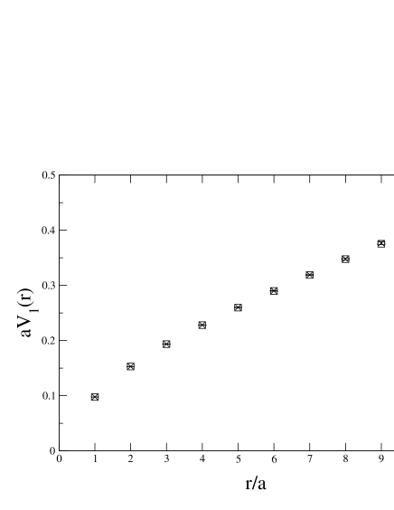
Figure 1: Singlet potential extracted from the Wilson loop $\langle W(r,t)\rangle$ (open squares), and correlations of dressed Wilson lines $\langle\tilde{L}({\bf x})\tilde{L}({\bf y})\rangle$ (crosses), for $\beta=9,L^{2}\cdot N_{t}=32^{3}$.

Next, we consider finite temperatures and dressed Polyakov loop correlations. The deconfinement transition of the 2+1 dimensional gauge theory has been studied in [15],[16]. The relationship between the inverse critical temperature in lattice units, $N_{t}^{c}=1/(aT_{c})$, and the lattice gauge coupling $\beta$ is well fitted by $N_{t}^{c}(\beta)=(\beta-0.37)/1.55$ [17]. For the following calculation of the static potentials we work at $\beta=9$, for which the deconfinement transition is between $N_{t}^{c}=5,6$. The three potentials are shown for decreasing temperatures in Fig. 2.

         

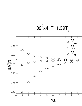
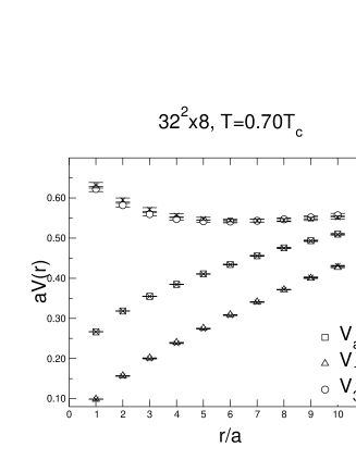
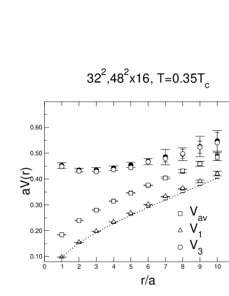
Figure 2: Singlet, triplet and average potentials calculated for different temperatures at $\beta=9$. At $T=0.7T_{c}$, the crosses denote data obtained in standard Coulomb gauge. At $T=0.35T_{c}$, filled symbols denote data obtained on a $48^{2}\cdot 16$ lattice. The dotted line marks the $T=0$ Wilson loop data from Fig. 1.

The results clearly confirm the perturbative expectation that the triplet potential is repulsive at short distances. In the deconfined phase all potentials assume a Yukawa form and merge at a common constant value at large distance, i.e. all color interactions are screened. In the confinement phase, however, the triplet potential becomes attractive at larger distances, while staying always above the singlet potential for the distances covered in the simulation. This is in accord with the fact that no stable charged states are observed empirically. Nevertheless, at low temperatures a potential well seems to form in which a metastable bound state appears possible. An investigation of this phenomenon in 4d SU(3) would be particularly interesting for heavy quark phenomenology, such as $J/\Psi$-production through an octet channel. A nice consistency check for the calculation is provided by comparing the singlet potential in the low temperature case with the zero temperature potential obtained from the Wilson loop. The latter is indicated in the figure for $T=0.35T_{c}$ by the dotted line, which is approached by the low $T$ Polyakov loop data from above, as expected on physical grounds.

As reported in [7], the non-locality of the functionals $\Omega[U]$ has them project predominantly on flux tubes encircling the periodic spatial volume, hampering the observation of localized states by large finite volume effects. Such effects are absent in the current calculations, as is demonstrated in Fig. 2 in the low $T$ plot, where the data for $L=32,48$ yield entirely consistent results. This is easily understood recalling that the quark-antiquark system is spatially extended, and the non-locality of the $\Omega(x)$ actually enables flux tubes to connect the pair over large distances. The flux represented by $\Omega(x)$ also closes through the periodic boundary conditions. As a consequence, we really measure a superposition of $\exp-N_{t}V(r)$ and $\exp-N_{t}V(L-r)$. However, for our choices of $N_{t},L$, the second term is exponentially suppressed compared to the first one, and no finite volume effects are observed.

In order to illustrate the independence of the calculation of the particular choice of $\Omega$, the $T=0.7T_{c}$ plot in Fig. 2 shows an additional calculation, where $\Omega[U]$ is the functional to fix standard Coulomb gauge, i.e. it minimizes the function $R[U]=\sum_{x,i}[1-1/N{\rm Tr\,}\Omega^{\dagger}(x)U_{i}(x)\Omega(x+\hat{\i})]$ in every timeslice. The corresponding data points, shown as crosses in the plot, coincide with those from the previous calculation. The reader is reminded that the lattice Coulomb gauge in principle is afflicted by Gribov copies. Since we know from our analytical considerations that the potentials have to be independent of the choice of $\Omega$, this numerical result may be interpreted as a test for the effect of Gribov copies in the standard Coulomb gauge.

Having separate non-perturbative results for the singlet and adjoint channel potentials, they should approach the leading order perturbative prediction, Eq. (2), in a regime where perturbation theory is valid. This is the case at short distances, and expected to extend to larger distances in the deconfined phase. Since the static potential includes an unphysical divergence which is different in continuum and lattice regularizations, we compare the physical forces $F_{i}=dV_{i}/dr$. Fig. 3 shows results obtained in the deconfined phase on a finer lattice, by employing the discretized forward derivative $F_{i}(r)=\Delta_{r}V_{i}(r)=(V_{i}(r+a)-V(r))/a$. Satisfactory agreement with the leading order perturbative result is observed.

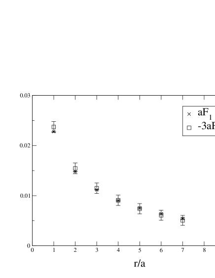
Figure 3: Comparison of the forces in the singlet and adjoint channels, computed at $\beta=18,L^{2}\cdot N_{t}=48^{2}\cdot 8$, corresponding to $T=1.42T_{c}$.

To conclude, in following the methods of [6, 7], we have shown that a dressed static quark-antiquark pair can exist in locally gauge invariant singlet and adjoint states, the latter transforming as a global $(N^{2}-1)$-plet. Calculation of the correspondingly dressed Polyakov loop correlation functions then permits the non-perturbative extraction of the singlet, adjoint and average potentials which are each eigenvalues of the Hamiltonian and hence gauge invariant. Numerical results for 2+1 d SU(2) gauge theory provide a consistent picture, in agreement with perturbation theory at small distances and large temperatures. Moreover, the calculation allows to observe how the finite temperature singlet potential extracted from the dressed Polyakov loop approaches the Wilson loop results in the zero temperature limit. The adjoint channel potential is repulsive at short distances. At zero temperature it becomes confining at large distances, allowing for a metastable bound state which should be of interest for heavy quark phenomenology. The considerations in this work can be applied to construct gauge invariant symmetric and antisymmetric quark-quark potentials as well. Apart from their relevance for heavy quark physics and the confinement problem, our results should also offer new ways to study the forces and excitations in hot and dense QCD.

Acknowledgements: I enjoyed useful discussions with O. Bär, Y. Schröder, B. Svetitsky and U.-J. Wiese. The simulations in this paper were performed on a NEC/SX-32 at the HLRS at the Universität Stuttgart, supported by the ITP, Universität Heidelberg.

References

- [1] L. S. Brown and W. I. Weisberger, Phys. Rev. D 20 (1979) 3239.
- [2] S. Nadkarni, Phys. Rev. D 34 (1986) 3904.
- [3] N. Attig et al., Phys. Lett. B 209 (1988) 65.
- [4] S. Necco and R. Sommer, Phys. Lett. B 523 (2001) 135.
- [5] L. D. McLerran and B. Svetitsky, Phys. Rev. D 24 (1981) 450.
- [6] O. Philipsen, Phys. Lett. B 521 (2001) 273.
- [7] O. Philipsen, hep-lat/0112047, to appear in Nucl. Phys. B.
-
[8]
A.M. Polyakov (ICTP, Trieste). IC-78-4-mc (microfiche), 64 pp., Feb 1978,
Lectures given at ICTP, Trieste, Nov. 1977;
G. ’t Hooft, Nucl. Phys. B 153 (1979) 141. - [9] K. G. Wilson, Phys. Rev. D 10 (1974) 2445.
- [10] J. C. Vink and U. Wiese, Phys. Lett. B 289 (1992) 122.
- [11] M. Creutz, Phys. Rev. D 15 (1977) 1128.
- [12] M. Lüscher, Commun. Math. Phys. 54 (1977) 283.
- [13] Y. Schröder, The static potential in at one loop, proceedings of ‘Strong and Electroweak Matter 97’, Eger, Hungary, World Scientific 1998, p.394.
- [14] P. de Forcrand and O. Philipsen, Phys. Lett. B 475 (2000) 280.
- [15] M. Teper, Phys. Lett. B 313 (1993) 417.
- [16] J. Engels, F. Karsch, E. Laermann, C. Legeland, M. Lütgemeier, B. Petersson and T. Scheideler, Nucl. Phys. Proc. Suppl. 53 (1997) 420.
- [17] A. Hart, B. Lucini, Z. Schram and M. Teper, JHEP 0006 (2000) 040.