hep-lat/0203013

The topological susceptibility of SU(3) gauge theory near $T_{c}$
Christof Gattringer^†, Roland Hoffmann and Stefan Schaefer Institut für Theoretische Physik, Universität Regensburg

D-93040 Regensburg, Germany

Abstract

We compute the topological susceptibility $\chi_{t}$ in SU(3) lattice gauge theory using fermionic methods based on the Atiyah-Singer index theorem. Near the phase transition we find a smooth crossover behavior for $\chi_{t}$ with values decreasing from (191(5) MeV)⁴ to (100(5) MeV)⁴ as we increase the temperature from 0.88 $T_{c}$ to 1.31 $T_{c}$, showing that topological excitations exist far above $T_{c}$. Our study is the first large scale analysis of the topological susceptibility at high temperature based on the index theorem and the results agree well with field theoretical methods.

To appear in Physics Letters B

PACS: 11.15.Ha
Key words: Lattice gauge theory, topology, index theorem

 

^† Supported by the Austrian Academy of Sciences (APART 654).

Relating topology to the dynamics of a gauge theory is a fascinating idea which can provide deep insights to the non-perturbative structure of the theory. For QCD an object of particular interest is the topological susceptibility $\chi_{t}$ defined as

$$\chi_{t}\;\;=\;\;\frac{1}{V}\;\langle Q^{2}\rangle\;.$$ (1)

$Q$ denotes the topological charge obtained e.g. as an integral over $F_{\mu\nu}\widetilde{F}_{\mu\nu}$. For QCD $\chi_{t}$ plays an important role in the low energy behavior where e.g. the so-called Witten-Veneziano formula [1] relates the quenched $\chi_{t}$ to the meson masses. For pure gauge theory $\chi_{t}$ is a measure for the net abundance of topological fluctuations and can provide insight to instanton liquid models [2]. Here the behavior around the phase transition is of particular interest, since new machines such as RHIC are starting to probe hot QCD. $\chi_{t}$ is expected to show a smooth crossover behavior into the high temperature phase as topological excitations die out.

The computation of $\chi_{t}$ near $T_{c}$ is an inherently non-perturbative calculation and can e.g. be attacked in lattice gauge theory. While for SU(3) lattice gauge theory at zero temperature there are several recent calculations [3]-[5], only a single modern study [5] of the critical behavior near $T_{c}$ can be found in the literature (for an early attempt see [6]). In this article we improve on this situation and present a systematic study of $\chi_{t}$ near the critical temperature with high statistics and an assessment of finite size effects from a comparison of data from different lattice sizes.

The traditional approach [3] to the calculation of the topological charge was a discretization of $F_{\mu\nu}\widetilde{F}_{\mu\nu}$ (the so-called field theoretical method). Lattice discretizations of $F_{\mu\nu}\widetilde{F}_{\mu\nu}$ are very sensitive to ultraviolet fluctuations and can be used only after some cooling or smearing procedure has been applied to the gauge field. Such a cooling step, however, has the potential to destroy topological lumps and to alter the outcome for $\chi_{t}$. Thus it is important to check whether there is consistency with alternative methods.

In this letter we compute the topological charge using a fermionic method (compare also [4, 7]). For the continuum Dirac operator $D$ the Atiyah-Singer index theorem [8] relates the topological charge $Q$ to the index of $D$ which can be written as the difference of the numbers of left-handed and right-handed zero-modes. For the standard Wilson-Dirac operator such a determination of $Q$ through the zero-modes fails for numerically accessible values of the cutoff since the would-be zero-modes mix with the corresponding modes in the doubler branches [9].

With the re-discovery of the Ginsparg-Wilson relation [10] for lattice Dirac operators it was understood how to formulate chirally symmetric fermions on the lattice. In particular Ginsparg-Wilson fermions give rise to an index theorem [11] already at finite cutoff. It was found [11, 12] that

$$Q\;\;=\;\;n_{-}\;-\;n_{+}\;\;=\;\;\frac{1}{2}\,\mbox{Tr}\,\gamma_{5}\,D\;\;=\;\;\frac{1}{32\pi^{2}}\int d^{4}xF_{\mu\nu}(x)\widetilde{F}_{\mu\nu}(x)\;+\;{\cal O}(a^{2})\;.$$ (2)

In the first line of the equation $n_{+}$ ($n_{-}$) denotes the number of zero-modes with positive (negative) chirality. The problem with the doublers is resolved since their would-be zero-eigenvalues are shifted to $2/a$. The great disadvantage of an exact solution of the Ginsparg-Wilson equation such as the overlap operator [13] is the high cost of a numerical implementation.

A possible, considerably cheaper approach is to use an approximate solution of the Ginsparg Wilson equation such as a finite parameterization of the fixed point action [14]. In this study we use chirally improved fermions [15] which arise from a systematic expansion of a solution of the Ginsparg-Wilson equation. They are sufficiently chiral to allow for an unambiguous identification of the zero-modes but are numerically considerably cheaper than overlap fermions and allow to obtain the statistics necessary for a precise measurement of $\chi_{t}$.

Our (quenched) SU(3) gauge configurations were generated with the Lüscher-Weisz action [16]. The leading coupling $\beta_{1}$ varied in a range from $\beta_{1}=8.10$ to $\beta_{1}=8.60$. When using the Sommer parameter $r_{0}=0.5$ fm to set the scale this corresponds [17] to a range of lattice spacings from $a=0.084$ fm to $a=0.125$ fm (compare Table 1 below). For details concerning the Monte Carlo see [18]. We used two settings of lattices: Firstly, $L^{4}$ lattices with $L=16$ and $L=12$. These ensembles are all in the low temperature phase of QCD, where quarks are confined and chiral symmetry is broken. Secondly, we use lattices of size $6\times L^{3}$ with $L=20,L=16$ and $L=12$. These latter ensembles give rise to temperatures ranging from values below the critical temperature (0.88 $T_{c}$) to values above the phase transition (1.31 $T_{c}$). The details for the parameters of our runs can be found in Table 1. For the Lüscher-Weisz action the critical temperature was computed in [19] using Polyakov loops and also the gap of the spectrum of the Dirac operator. Both the chiral transition and the deconfinement transition were found to have a critical temperature of $T_{c}=300(3)$ MeV.

lattice	$\beta_{1}$	$a$ [fm]	$T$ [MeV]	$N_{confs}$	$\chi_{t}^{\frac{1}{4}}$ [MeV]
$6\times 20^{3}$	8.10	0.125(1)	264(2)	400	194(5)
$6\times 20^{3}$	8.20	0.115(1)	287(3)	400	185(5)
$6\times 20^{3}$	8.25	0.110(1)	299(3)	400	162(5)
$6\times 20^{3}$	8.30	0.106(1)	311(3)	400	144(5)
$6\times 20^{3}$	8.45	0.094(1)	350(4)	400	124(5)
$6\times 20^{3}$	8.60	0.084(1)	392(5)	400	93(5)
$6\times 16^{3}$	8.10	0.125(1)	264(2)	800	200(4)
$6\times 16^{3}$	8.20	0.115(1)	287(3)	800	186(4)
$6\times 16^{3}$	8.25	0.110(1)	299(3)	800	170(4)
$6\times 16^{3}$	8.30	0.106(1)	311(3)	800	153(4)
$6\times 16^{3}$	8.45	0.094(1)	350(4)	800	123(4)
$6\times 16^{3}$	8.60	0.084(1)	392(5)	800	105(5)
$6\times 12^{3}$	8.10	0.125(1)	264(2)	1200	191(4)
$6\times 12^{3}$	8.20	0.115(1)	287(3)	1200	183(4)
$6\times 12^{3}$	8.25	0.110(1)	299(3)	1200	170(4)
$6\times 12^{3}$	8.30	0.106(1)	311(3)	1200	153(4)
$6\times 12^{3}$	8.45	0.094(1)	350(4)	1200	118(4)
$6\times 12^{3}$	8.60	0.084(1)	392(5)	1200	101(5)
$16^{4}$	8.10	0.125(1)	99(1)	200	185(6)
$16^{4}$	8.20	0.115(1)	107(1)	200	194(7)
$16^{4}$	8.30	0.106(1)	117(1)	200	189(6)
$16^{4}$	8.45	0.094(1)	131(1)	200	194(6)
$16^{4}$	8.60	0.084(1)	147(2)	200	192(7)
$12^{4}$	8.10	0.125(1)	132(1)	400	200(5)
$12^{4}$	8.30	0.106(1)	155(1)	400	188(5)
$12^{4}$	8.45	0.094(1)	175(2)	400	191(5)

Table 1: Parameters and results. We give the size of our lattices, the inverse gauge coupling $\beta_{1}$, the corresponding lattice spacing $a$ in fermi, the temperature in MeV, the number $N_{confs}$ of configurations in our ensembles and our results for the topological susceptibility.

Since the chirally improved fermions we are using here are only an approximation of a solution of the Ginsparg-Wilson equation a few comments on our determination of the topological charge are in order here. One of the effects of using an approximation of a Ginsparg-Wilson operator are fluctuations of the zero-eigenvalues. Instead of being located exactly at the origin the zero-eigenvalues manifest themselves as small real eigenvalues. It can be demonstrated [20] that for discretized instantons the size of these would-be zero-eigenvalues increases as the radius of the instanton decreases. Similarly, also for the thermalized configurations one finds a distribution of real eigenvalues. For two of our ensembles ($16^{4}$ and $6\times 20^{3}$ both at $\beta_{1}=8.20$) we show this distribution in Fig. 1. The distribution of the position $x$ of the real eigenvalues has a pronounced peak at the origin and a tail which extends towards larger values. The tail comes from very small instantons, so-called dislocations.

Figure 1: Distribution of the real eigenmodes of the chirally improved Dirac operator for the $\beta=8.20$ ensembles. The dashed histogram represents the data from the $16^{4}$ lattice while the full line is for $6\times 20^{3}$.

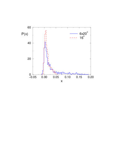
We compute our eigenvalues using the implicitly restarted Arnoldi method [21]. This algorithm computes a given number $N$ of eigenvalues ordered with respect to their absolute value. We always compute the $N=50$ smallest eigenvalues, except for the $16^{4}$ lattices where we have $N=30$. A potential source of error is a too low value of $N$. Sufficiently many eigenvalues have to be computed in order to capture all of the peak in the distribution of Fig. 1. As is obvious from Fig. 1 with our choice of $N$ we obtain all of the peak and a large portion of the tail. Setting a cut for the eigenvalues at e.g. 0.1 leaves the results for $\chi_{t}$ unchanged showing that dislocations make up only a small contribution to the topological susceptibility. We remark that there is no danger of mistaking a would-be zero eigenvalue for an eigenvalue with a small but non-vanishing imaginary part. A few lines of algebra [22] show that for a $\gamma_{5}$-hermitian Dirac operator the matrix element $\psi^{\dagger}\gamma_{5}\psi$ of an eigenvector $\psi$ is non-zero only for eigenvectors with real eigenvalues. For our approximation of a Ginsparg-Wilson Dirac operator we find values of $|\psi^{\dagger}\gamma_{5}\psi|$ ranging from 0.8-0.9 in the peak of the distribution down to 0.4 for the very end of the tail.

We summarize our procedure for determining $Q$ as follows: We compute the 50 (30 for $16^{4}$) eigenvalues of the Dirac operator and for the eigenvectors with real eigenvalues evaluate $\psi^{\dagger}\gamma_{5}\psi$. We take $n_{+}$ ($n_{-}$) to be the number of modes where $\psi^{\dagger}\gamma_{5}\psi$ is positive (negative). The topological charge is then computed as in Eq. (2) by $Q=n_{-}-n_{+}$.

For a subsample of 200 configurations on the $12^{4}$ lattices at $\beta_{1}=8.10$ and $\beta_{1}=8.45$ we cross-checked our procedure with the results obtained from the overlap operator. For the overlap operator the zero-modes have eigenvalues exactly at zero since also modes from dislocations are projected onto exact zero-modes. The corresponding $\gamma_{5}$ matrix elements are always $\psi^{\dagger}\gamma_{5}\psi=\pm 1$. When comparing the determination of $Q$ for the individual configurations we found a discrepancy for 2% for the configurations at $\beta_{1}=8.45$ and 9% for $\beta_{1}=8.10$. This demonstrates that as one goes closer to the continuum limit the two definitions agree better. Furthermore, the difference in $Q$ was always only one unit such that the results for $\chi_{t}$ agree surprisingly well: For the subsamples of 200 configurations we found at $\beta_{1}=8.45$ a value of $\chi_{t}=$ (182 (7) MeV)⁴ for both methods. At $\beta_{1}=8.10$ we obtained a value of $\chi_{t}=$ (196 (7) MeV)⁴ with the overlap operator and $\chi_{t}=$ (197 (7) MeV)⁴ with the chirally improved operator. Our test shows that the two methods agree very well, however, using the overlap operator is by a factor of 10 more costly than working with the chirally improved operator. We remark that a direct comparison of the field theoretical approach and the fermionic method on single configurations can be found in [7].

Figure 2: The topological susceptibility as a function of $\beta$. We show our results for the zero temperature ensembles on $12^{4}$ (circles) and $16^{4}$ (filled circles) as well as for the finite temperature ensembles on $6\times 12^{3},6\times 16^{3}$ and $6\times 20^{3}$ lattices (squares, triangles, diamonds). The dashed vertical line marks the phase transition.

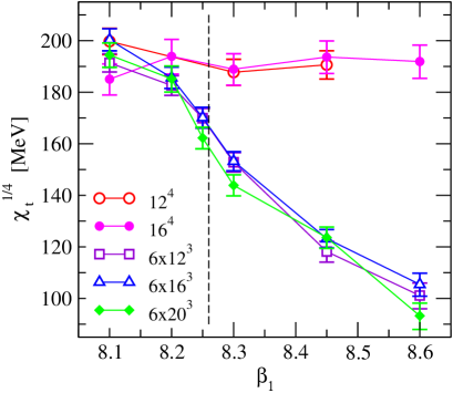
We begin with a discussion of the results for $\chi_{t}$ as a function of $\beta_{1}$. We plot the corresponding data in Fig. 2. For time extent 6 the critical value of $\beta_{1}$ was determined [19] to be $\beta_{1}=8.26(2)$. We mark the transition with a dashed vertical line in Fig. 2. For the $6\times L^{3}$ configurations we used values of $\beta_{1}$ ranging from $8.10$ to $8.60$ giving rise to ensembles on both sides of the transition. The corresponding data are represented in Fig. 2 by squares ($6\times 12^{3}$), triangles ($6\times 16^{3}$) and diamonds ($6\times 20^{3}$). We connect the symbols to guide the eye. When comparing the results for different volumes we find that the data agree well within error bars. This shows that for the chosen lattice sizes we do not encounter finite size problems. For $\beta_{1}=8.10$ our values for $\chi_{t}$ scatter around (190 MeV)⁴, which is the value in the low temperature phase. As one increases $\beta_{1}$, $\chi_{t}$ starts to drop already before the critical value $\beta_{1}=8.26$ is reached. The slope of the curve is largest near the critical $\beta_{1}$. The decrease slows down as $\beta_{1}$ is increased further and $\chi_{t}$ reaches a value of $\chi_{t}\sim$ (100 MeV)⁴ at $\beta_{1}=8.60$.

The decreasing curve for $\chi_{t}$ from the ensembles at high temperature can now be compared to the low temperature data with the same values of $\beta_{1}$, i.e. the same cutoff. The corresponding data are represented by open circles ($12^{4}$) and filled circles ($16^{4}$). Again we find that the data from the two different volumes are well consistent within error bars and we do not face finite size problems. The numbers for $\chi_{t}$ remain near (190 MeV)⁴ for all values of $\beta_{1}$.

It is interesting to combine the results from the zero temperature ensembles and compare them to the results available in the literature. The combined result from our $16^{4}$ lattices is $\chi_{t}=$ (191(5) MeV)⁴. The more recent results in the literature range between $\chi_{t}=$ (175(5) MeV)⁴ to $\chi_{t}=$ (203(5) MeV)⁴. This demonstrates that our zero temperature result for the Lüscher-Weisz action determined from the index theorem agrees well with published data.

Figure 3: The topological susceptibility as a function of the temperature. We combine our results from all lattices: $12^{4},16^{4},6\times 12^{3},6\times 16^{3}$ and $6\times 20^{3}$ (circles, filled circles, squares, triangles, diamonds). The dashed vertical line marks the phase transition.

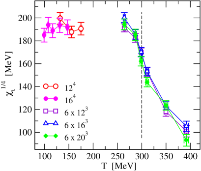
Let us now return to the more interesting behavior near the phase transition. In Fig. 3 we present our data as a function of the temperature. We include also our data for the $L^{4}$ lattices in order to have the baseline in the low temperature phase. The data from our high temperature, $6\times L^{3}$ configurations cover a temperature range from 264 MeV to 392 MeV. Again we mark the phase transition by a vertical dashed line. As already mentioned above, the data from different volumes agree very well and we do not encounter finite size problems. The topological susceptibility starts to deviate from its zero temperature value ($\chi_{t}\sim$ (190 MeV)⁴) at a temperature of $T\sim 275$ MeV which is still below the deconfinement transition. The drop continues and becomes steepset at $T_{c}$ and then leans back slightly. At our largest temperature $T=$ 392 MeV (= 1.31 $T_{c}$) the decrease is still substantial and $\chi_{t}$ has reached $\chi_{t}\sim$ (100 MeV)⁴ which is about half of its zero temperature value. A linear extrapolation of the decrease of $\chi_{t}^{1/4}$ gives a temperature of about 600 MeV where $\chi_{t}$ becomes compatible to zero. This would be about twice the critical temperature, but since the decrease of $\chi_{t}^{1/4}$ is certainly not linear throughout, $\chi_{t}\sim 0$ is presumably reached at a temperature even higher than 600 MeV. Our data are in reasonably well agreement with the other result for $\chi_{t}$ near $T_{c}$ available in the literature [5].

In this letter we have performed the first large scale study of the finite temperature behavior of $\chi_{t}$ based on the index theorem. Fermionic methods provide an alternative approach free from possible ambiguities due to cooling or smearing. From a comparison of data on different volumes we find that finite size effects are under good control. We find that the topological susceptibility extends into the high temperature phase and some topological excitations can be found up to 2 $T_{c}$.

Acknowldegements: We would like to thank Stefan Dürr, Meinulf Göckeler, Christian Lang, Paul Rakow and Andreas Schäfer for discussions. The calculations were done on the Hitachi SR8000 at the Leibniz Rechenzentrum in Munich and we thank the LRZ staff for training and support.

References

- [1] E. Witten, Nucl. Phys. B 156 (1979) 269; G. Veneziano, Nucl. Phys. B 159 (1979) 213.
- [2] D. Diakonov, Talk given at International School of Physics, ’Enrico Fermi’, Course 80: Selected Topics in Nonperturbative QCD, Varenna, Italy, 1995, hep-ph/9602375; T. Schäfer and E.V. Shuryak, Rev. Mod. Phys. 70 (1998) 323.
- [3] D. A. Smith and M. J. Teper [UKQCD collaboration], Phys. Rev. D 58 (1998) 014505; P. de Forcrand, M. Garcia Perez, J. E. Hetrick and I. O. Stamatescu, hep-lat/9802017; A. Hasenfratz and C. Nieter, Phys. Lett. B 439 (1998) 366.
- [4] R. G. Edwards, U. M. Heller and R. Narayanan, Nucl. Phys. B 535 (1998) 403; Nucl. Phys. Proc. Suppl. 73 (1999) 500; P. Hasenfratz, S. Hauswirth, K. Holland, T. Jörg and F. Niedermayer, Nucl. Phys. Proc. Suppl. 106 (2002) 751.
- [5] B. Allés, M. D’Elia, A. Di Giacomo, Nucl. Phys. B 494 (1997) 281.
- [6] M. Teper, Phys. Lett.B 202 (1988) 553.
- [7] J. B. Zhang, S. O. Bilson-Thompson, F. D. Bonnet, D. B. Leinweber, A. G. Williams and J. M. Zanotti, hep-lat/0111060.
- [8] M. Atiyah and I.M. Singer, Ann. Math 93 (1971) 139.
- [9] C. Gattringer and I. Hip, Nucl. Phys. B 541 (1999) 305, Nucl. Phys. B 536 (1998) 363; C. Gattringer, I. Hip and C. B. Lang, Nucl. Phys. Proc. Suppl. 63 (1998) 498.
- [10] P. H. Ginsparg and K. G. Wilson, Phys. Rev. D 25 (1982) 2649.
- [11] P. Hasenfratz, V. Laliena and F. Niedermayer, Phys. Lett. B 427 (1998) 125.
- [12] M. Lüscher, Phys. Lett. B 428 (1998) 342, Nucl. Phys. B 538 (1999) 515.
- [13] R. Narayanan and H. Neuberger, Phys. Lett. B 302 (1993) 62, Nucl. Phys. B 443 (1995) 305.
- [14] P. Hasenfratz, Nucl. Phys. B (Proc. Suppl.) 63 (1998) 53; P. Hasenfratz, Nucl. Phys. B 525 (1998) 401; P. Hasenfratz, S. Hauswirth, K. Holland, Th. Jörg, F. Niedermayer, U. Wenger, Int. J. Mod. Phys. C 12 (2001) 691; P. Hasenfratz, S. Hauswirth, K. Holland, T. Jörg and F. Niedermayer, Nucl. Phys. Proc. Suppl. 106 (2002) 799.
- [15] C. Gattringer, Phys. Rev. D 63 (2001) 114501; C. Gattringer, I. Hip, C.B. Lang, Nucl. Phys. B597 (2001) 451; C. Gattringer and I. Hip, Phys. Lett. B 480 (2000) 112.
- [16] M. Lüscher and P. Weisz, Commun. Math. Phys. 97 (1985) 59; Err.: 98 (1985) 433; G. Curci, P. Menotti and G. Paffuti, Phys. Lett. B 130 (1983) 205, Err.: B 135 (1984) 516.
- [17] C. Gattringer, R. Hoffmann and S. Schaefer, Phys. Rev. D, in print (hep-lat/0112024).
- [18] C. Gattringer, M. Göckeler, P.E.L. Rakow, S. Schaefer and A. Schäfer, Nucl. Phys. B 617 (2001) 101, Nucl. Phys. B 618 (2001) 205.
- [19] C. Gattringer, P.E.L. Rakow, A. Schäfer and W. Söldner, hep-lat/0202009.
- [20] C. Gattringer, M. Göckeler, C. B. Lang, P.E.L. Rakow, A. Schäfer, Phys. Lett. B 522 (2001) 194.
- [21] D.C. Sorensen, SIAM J.Matrix Anal.Appl.13 (1992) 357.
- [22] S. Itoh, Y. Iwasaki and T. Yoshie, Phys. Rev. D 36 (1987) 527; Phys. Lett. 184 B (1987) 375.