Scaling laws for the 2d 8-state Potts model with Fixed Boundary Conditions

Abstract

We study the effects of frozen boundaries in a Monte Carlo simulation near a first order phase transition. Recent theoretical analysis of the dynamics of first order phase transitions has enabled to state the scaling laws governing the critical regime of the transition. We check these new scaling laws performing a Monte Carlo simulation of the 2d, 8-state spin Potts model. In particular, our results support a pseudo-critical $\beta(L)$ finite-size scaling of the form $\beta(\infty)+a_{1}/L+a_{2}/L^{2}$, instead of $\beta(\infty)+\theta_{1}/L^{d}+\theta_{2}/L^{2d}$. Moreover, we obtain a latent heat, $\Lambda_{\rm FBC}=0.294(11)$, which does not coincide with the latent heat analytically derived for the same model if periodic boundary conditions are assumed, $\Lambda_{\rm PBC}=0.486358\ldots$

I Introduction

The introduction of computer simulation methods has been a breakthrough in the study of phase transitions in lattice models. The rapid increase on the computers power has enabled to analyze with great accuracy the scaling laws, governed by the critical exponents, and even the corrections to these scaling laws. In such analysis, finite size effects must be taken into account carefully Binder . One of these effects, the disturbance from the boundary, has usually been dismissed by the adoption of periodic boundary conditions (PBC). Nevertheless, in some situations the adoption of periodic lattices may not be adequate, either for practical or theoretical reasons. This is the case of the free boundary conditions used in the analysis of free surfaces, or the so called boundary fields, used in the analysis of wetting phenomena. In the present paper we will focus on a particular election of the boundary conditions, the so called fixed boundary conditions (FBC), which have been recently applied to spin models BEJ ; BEJ2 and gauge models BF .

Second order phase transitions exhibit universality. For this reason, all the details of the system near the phase transition point become irrelevant for the critical exponents. By contrast, first order phase transitions are not universal and, hence, all details of a simulation must be considered carefully. This includes, in particular, the choice of boundary conditions. What are the appropriate set of scaling laws for a first order phase transition with FBC? This is the question we address in this paper. Starting from the theoretical analysis of Borgs and Kotecky BK ; BK2 and the diploma Thesis of Medved M on the dynamics of first order transitions, we present the finite size scaling laws applicable to the case of FBC and we check them performing a numerical simulation of the 2-d 8-state spin Potts model Potts with FBC.

The paper is divided as follows. In section II a brief summary of some recent simulations where FBC have been adopted serves as a motivation for a detailed analysis of the finite size scaling laws which are also presented and discussed. Section III is devoted to a discussion of our numerical simulation and the results that we have obtained. In section IV we analyze our results in the light of the scaling laws presented in Sec. II. Finally, in section V we give some concluding remarks.

II Fixed Boundary Conditions

II.1 The motivation for FBC

Recently, the so called gonihedric spin modelshave been proposed as a laboratory to study discrete versions of string theories SW . All these simulations have been performed imposing standard periodic boundary conditions on a three-dimensional lattice. Nevertheless, in some cases three intersecting inner planes of spins were fixed to break the large energy degeneracy of the hamiltonianBEJ ; BEJ2 . Due to the periodicity of the boundaries, this is equivalent to fix the spins belonging to the six planes of the 2-d boundary of the 3-d cube formed by the spins. Since for a certain range of the coupling parameter, in particular for $\kappa=0$, the transition is clearly of first order, the analysis of the finite size effects should have been done using the scaling laws presented in this paper. We expect that the application of the FBC scaling laws may overcome some anomalies recently observed in the analysis of this transition BV .

Another situation where the knowledge of the FBC scaling laws seems to be crucial is the issue of the triviality of lattice QED. Indeed, it has been claimed that the formation of artificial monopole structures, which close over the boundaries, in a simulation of the 4-d U(1) gauge model may be responsible for turning the phase transition of this model from second to first order LJ . To avoid this problem, originated probably by an incorrect choice of the boundaries, it was suggested to perform the Monte Carlo simulations on a lattice with a topology of an sphere. Along these lines, Baig and FortBF proposed the adoption of FBC to simulate an spherical topology. Effectively, to fix all the variables belonging to the 3-d border to unity is the higher dimensional equivalent of converting a 2-d plane square lattice to the 2-d surface of a sphere by collapsing the lines of the border to a single point. Nevertheless, to discriminate between a first or a second order nature for a transition, an accurate analysis of data produced is necessary, and, in particular, this will be only possible if one knows for certain the applicable scaling laws.

II.2 The scaling laws

Although speaking properly no critical exponents can be defined for first order phase transitions, it is usual to define a set of characteristic exponents, together with a set of scaling laws borrowed from those of the second order phase transitions. The pioneering work of Privman and Fisher Privman , Binder and Landau Binder2 and Challa et al. Challa , provided a phenomenological understanding of the scaling for first order transitions. A more rigorous theoretical justification for these first order scaling laws was presented by Borgs and Kotecky BK ; BK1 . The formulation of its applicability to finite size scaling expressions in terms of the lattice size was the work of Borgs, Kotecky and Miracle-Solé BKS and, independently, of Janke Janke . But in all these developments the existence of periodic boundary conditions was assumed. Recently, though, Borgs and Kotecky BK2 have extended their analysis to include surface effects in addition to the standard volume effects which govern first order transitions. Following this work, Mendev M has deduced the scaling laws for the spin Potts model in the presence of surface effects, in particular adopting boundary conditions other than the periodic ones.

Following the general analysis of Mendev M , finite size scaling laws in terms of the lattice size for the case of fixed boundary conditions can easily be deduced. They are summarized in Table 1, together with the standard laws for periodic conditions. In the rest of this paper we will check these modified scaling laws with the results of our numerical simulation.

It should be noticed that the suggestion that in the case of free boundary conditions every transition is shifted by a $1/L$ correction term caused by surface effects is quite old. Binder Binder3 , for instance, reports on a series of experimental results Experiments supporting this conclusion.

Table 1: Scaling laws for Periodic and Fixed Boundary Conditions.

	P.B.C.	F.B.C.
$\beta_{c}^{peaks}(L)=$	$\beta_{c}(\infty)+\frac{\theta_{1}}{L^{d}}+O(\frac{1}{L^{2d}})$	$\beta_{c}(\infty)+\frac{a_{1}}{L}+O(\frac{1}{L^{2}})$
$C_{max}(L)=$	$\gamma_{0}+\gamma_{2}L^{d}+O(\frac{1}{L^{d}})$	$c_{0}+c_{2}L^{d}+O(L^{d-1})$
$\chi_{max}(L)=$	$\delta_{0}+\delta_{2}L^{d}+O(\frac{1}{L^{d}})$	$e_{0}+e_{2}L^{d}+O(L^{d-1})$
$B_{min}(L)=$	$\Phi_{0}+\frac{\Phi_{1}}{L^{d}}+O(\frac{1}{L^{2d}})$	$B_{0}+\frac{B_{1}}{L}+O(\frac{1}{L^{2}})$

III Numerical simulation

To test the scaling laws of Table 1, we have performed a numerical simulation of the 2-d 8-state spin Potts model defined by the partition function

$$Z_{potts}=\sum_{\{\sigma_{i}\}}e^{-\beta E},$$ (1)

where the energy is

$$E=-\sum_{\langle ij\rangle}\delta_{\sigma_{i}\sigma_{j}},\;\;\;\;\;(\sigma_{i}=1,...,8),$$ (2)

with $\beta=J/kT$ in natural units. It is well known that this model exhibits a first order phase transition Wu and for this reason it has been chosen as a test model in several previous studies.

Fixed boundary conditions have been implemented along the lines stated by Baig and Fort BF . In a 2-d grid with points labeled by $(n_{x},n_{y})$, all spins corresponding to the lattice points $(1,n_{y})$ and $(n_{x},1)$ for $n_{x},n_{y}=1,...,L$ have been fixed during all the simulation at its initial values $\sigma=1$. With this precaution, the structure of the program, that implements PBC, assures the persistence of the frozen boundary.

We have performed the lattice updating applying a well tested head bath algorithm. During the simulation we recorded time series files for the energy $E$ and the magnetization $M$ defined as

$$M=\frac{q\;\mbox{max}\{n_{i}\}-L^{d}}{q-1},$$ (3)

where $q=8$ and $n_{i}$ is the number of spins in a given orientation.

Table 2 summarizes the details of the simulations that have performed from $L=70$ up to $L=350$. The number of production Monte Carlo sweeps varies from $n_{\rm prod}=6~{}000~{}000$ for $L=70$, to $n_{\rm prod}=32~{}700~{}000$ for $L=350$. Since we took measurements only every $n_{\rm flip}=8$ sweeps, the number of total measurements per run is $n_{\rm meas}=n_{\rm prod}/n_{\rm flip}$. We left at least $20\,n_{\rm flip}\tau_{\rm e}$ thermalization sweeps before taking measurementsSokal ; Sokal2 ; Janke2 . To estimate the autocorrelation time of energy measurements $\tau_{\rm e}$, we have applied two different methods. First, we use the fact that $\tau_{\rm e}$ enters the error estimate $\epsilon_{\rm JK}=\sqrt{2\;\tau_{\rm e}/n_{\rm meas}}\,\epsilon_{\rm naive}$ for the mean energy $<E>$ of $n_{\rm meas}$ correlated energy measurements of variance

$$\epsilon_{\rm naive}^{2}=\sum_{j=1}^{n_{\rm meas}}(<E>-E_{j})^{2}/(n_{\rm meas}-1).$$

The “true” error estimate $\epsilon_{\rm JK}$ is obtained splitting the energy time-series into 50 bins, which were in their turn jackknived jack ; jack2 to decrease the bias in the analysis. The second way of obtaining $\tau_{\rm e}$ is by a direct computation of the integrated autocorrelation time

$$\tau_{e}^{\rm int}=\frac{1}{2}+\sum_{j=1}^{k_{\rm max}-1}(1-j/k_{\rm max})\frac{\frac{1}{k_{\rm max}-(j-1)}\;\sum_{i=1}^{k_{\rm max}-(j-1)}(E_{i}-<E>)(E_{i+j}-<E>)}{<E^{2}>-<E>^{2}},$$

where $k_{\rm max}$ is a suitable cut-off Sokal around $6\,\tau_{e}^{\rm int}<k_{\rm max}<10\,\tau_{e}^{\rm int}$. The corresponding error in $\tau_{e}^{\rm int}$ is derived from the a priori formula $\sqrt{2\,(2\,k_{\rm max}+1)/n_{\rm meas}}\,\tau_{e}^{\rm int}$.

Table 2: Monte Carlo parameters of the simulation. $L^{2}$ is the lattice size, $n_{\rm therm}$ the number of Monte Carlo sweeps during thermalization, and $n_{\rm prod}$ the number of production runs. Measurements were taken every $n_{\rm flip}=8$ Monte Carlo sweeps for all the simulations.

$L$	$\beta_{MC}$	$n_{\rm therm}$	$n_{\rm prod}$	$\tau_{\bf\rm e}$	$\tau_{\bf\rm e}^{\rm int}$	$\frac{n_{\rm therm}/n_{\rm flip}}{\tau_{\bf\rm e}}$	$\frac{n_{\rm prod}/n_{\rm flip}}{2\,\tau_{\bf\rm e}}$
70	1.3343	100 000	6 000 000	144	128(12)	87	2604
84	1.3363	100 000	6 000 000	208	240(25)	60	1803
100	1.3378	150 000	8 000 000	357	394(38)	53	1441
126	1.33909	250 000	8 000 000	883	847(122)	35	567
150	1.3398	400 000	10 000 000	1320	1341(215)	38	474
200	1.3407	900 000	12 000 000	4664	5434(1582)	24	161
226	1.34102	1 200 000	16 000 000	7287	6991(1476)	21	138
250	1.341205	1 600 000	18 000 000	9072	9700(2454)	22	124
278	1.34138	2 200 000	18 800 000	11743	16969(5058)	23	100
300	1.34146	3 000 000	22 000 000	15429	27765(12969)	24	89
350	1.34162	4 000 000	32 700 000	25632	53623(29055)	20	80

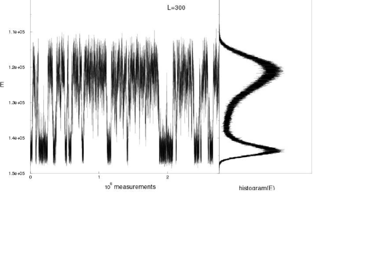
Figure 1: Energy time series for $L=300$ and $\beta_{MC}=1.34146$

In Fig. 1 we present the energy time-series for the $L=300$ and $\beta_{MC}=1.34146$ simulation run. The expected characteristic behaviour for a first order phase transition can be clearly seen. The system remains in one of the two coexisting phases for a long period of time. The energy histogram for the full series is also presented in this figure. The similar height of the two peaks confirms that the simulation was performed very near the pseudo-critical inverse temperature.

It is instructive to compare the energy histograms corresponding to the adoption of fixed or periodic boundary conditions. To this end we have performed two different Monte Carlo runs, close to the respective pseudo-critical inverse temperatures, which are $\beta_{MC}^{PBC}=1.342027$ and $\beta_{MC}^{FBC}=1.3378$ for a lattice size $L=100$. These simulations has been done using $8~{}000~{}000$ production sweeps, with $n_{\rm flip}=8$, discarding the initial $250000$ ($150000$) sweeps in the case of PBC (FBC) for the thermalization of the system. Both histograms can be seen in Fig. 2. They show the characteristic two-peaks structure. Nevertheless, the latent heat, i.e., the separation between the maximum of the two peaks, is clearly smaller for Fixed Boundary Conditions. This qualitative observation suggest that a simple analysis of the energy histograms of a true first order phase transition simulated with Fixed Boundary Conditions might be misleading. Effectively, if the lattice size is not large enough the energy histogram could show (apparently) a single peak and, in consequence, one can get the erroneous conclusion that the model exhibit a second order phase transition. Nevertheless, even with FBC the evolution of the energy histograms when the size of the system increases shown in Fig. 2 ($L=100$), and in Fig.1 ($L=300$), exhibit the expected behaviour of a first order transition. This observation may be relevant in the interpretation of the analysis of Baig and Fort BF , where a disappearance of a two peaks structure was observed when FBC were imposed to the system N1 .

In addition to the qualitative analysis of the histograms, we have computed the specific heat, magnetic susceptibility and the Binder kurtosis parameter at nearby values of $\beta_{MC}$ by means of standard reweighting techniques Swendsen . They are defined as

$$C(\beta) = \frac{\beta^{2}}{L^{2}}(\langle E^{2}\rangle-\langle E\rangle^{2}),$$ (4)

$$\chi(\beta) = \frac{\beta^{2}}{L^{2}}(\langle M^{2}\rangle-\langle M\rangle^{2}),$$ (5)

$$B(\beta) = 1-\frac{\langle E^{4}\rangle}{3\langle E^{2}\rangle^{2}}.$$ (6)

In table 3 we show the extrema of the magnitudes above defined, together with their pseudo-critical inverse temperatures. The error bars of these quantities have been estimated splitting the time-series data into 50 bins, which were jackknived to decrease the bias in the analysis of reweighted data.

Table 3: Extrema for the (finite lattice) specific heat, $C_{\rm max}$, the susceptibility, $\chi_{\rm max}$, and the energetic Binder parameter, $B_{\rm min}$, together with their respective pseudo-critical inverse temperatures.

$L$	$\beta_{\rm max}^{C}$	$C_{\rm max}$	$\beta_{\rm max}^{\chi}$	$\chi_{\rm max}$	$\beta_{\rm min}^{B}$	$B_{\rm min}$
70	1.334469(53)	89.26(96)	1.334212(52)	95.3(1.2)	1.333966(52)	0.660221(74)
84	1.336360(46)	124.6(1.4)	1.336215(45)	143.8(1.7)	1.336040(46)	0.660441(71)
100	1.337705(34)	171.3(1.9)	1.337620(33)	210.5(2.5)	1.337492(33)	0.660657(69)
126	1.339124(33)	268.4(4.1)	1.339081(33)	355.8(5.7)	1.339000(33)	0.660774(94)
150	1.339905(25)	391.5(7.4)	1.339881(25)	550(11)	1.339821(25)	0.66058(12)
200	1.340747(23)	757(16)	1.340739(22)	1144(25)	1.340704(22)	0.66006(15)
226	1.341046(18)	1006(27)	1.341042(18)	1554(43)	1.341014(18)	0.65981(19)
250	1.341229(15)	1285(29)	1.341225(15)	2033(47)	1.341203(15)	0.65950(17)
278	1.341379(12)	1695(42)	1.341377(12)	2735(69)	1.341358(12)	0.65900(20)
300	1.341493(12)	2083(51)	1.341491(12)	3413(86)	1.341475(12)	0.65856(21)
350	1.3416496(92)	3176(77)	1.3416490(92)	5338(130)	1.3416373(92)	0.65754(23)

IV Scaling laws analysis

Once we have the results from the numerical simulation on finite lattices, we can proceed to analyze the data imposing the scaling laws of Table 1.

IV.1 Analysis of the pseudo-critical inverse temperature

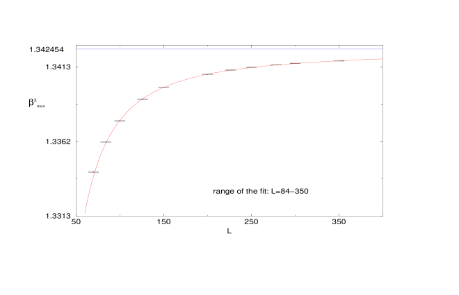
Figure 3: Finite-size scaling analysis of the pseudo-critical $\beta^{\chi}_{\rm max}$ in the range $L=84-350$ by means of the ansatz $\beta^{\chi}_{\rm max}(L)=\beta_{c}+\alpha_{1}/L+\alpha_{2}/L^{2}$. The infinite volume critical point obtained from the fit is $\beta_{c}=1.342478(38)$, with a goodness-of-fit $Q=0.13$.

In Table 4 we present the results of fitting the pseudo-critical betas of $C_{\rm max}$, $\chi_{\rm max}$ and $B_{\rm min}$ to the ansatz $\beta_{c}+a_{1}/L+a_{2}/L^{2}$ suggested by the finite-size scaling laws presented in Table 1. Notice that we have performed two set of fits, one for the full range $84\leq L\leq 350$, and a second including only results from the lattice sizes $100\leq L\leq 350$. Notice that the fits are extremely good even for the initial range $84\leq L\leq 350$, but they improve slightly if $L=84$ is discarded. Remember that reasonable fits should have a goodness-of-fit NR , $Q$, above 0.05. Fig. 3 depicts the fit for $\beta_{\chi}^{\rm max}(L)$ in the range $84\leq L\leq 350$. The exact critical inverse temperature for the 2d 8-state Potts model is $\beta_{c}(exact)=\ln(1+\sqrt{(}8))=1.342454\ldots$. Our results of Table 4 are in perfect agreement with this value.

We have also fitted our data to the ansatz $\beta^{peaks}_{c}=\beta(\infty)+\theta_{1}/L^{2}+\theta_{2}/L^{4}$ corresponding to the PBC finite-size scaling law. Even though the goodness-of-fit, $Q$, obtained does not allow to discard the fits, the infinite volume $\beta_{c}(\infty)$ resulting from them do not coincide with the exactly known value, showing that this ansatz is unsuitable. I.e. for the $\beta^{C}_{\rm max}(L)$ in the range $84\leq L\leq 350$, the fit produces $Q=0.10$ and $\beta_{c}(\infty)=1.342063(11)$ and for $\beta^{\chi}_{\rm max}(L)$ in the range $100\leq L\leq 350$, the results are $Q=0.21$ and $\beta_{c}(\infty)=1.342079(13)$.

Table 4: Pseudo-critical inverse temperature fits. Q is the goodness-of-fit. Recall that the exact critical inverse temperature for the model is $\beta_{c}(exact)=\ln(1+\sqrt{(}8))=1.342454\ldots$

range L’s	$\beta^{C}_{\rm max}(L)=\beta_{c}+a_{1}/L+a_{2}/L^{2}$				$\beta^{\chi}_{\rm max}(L)=\beta_{c}+a_{1}/L+a_{2}/L^{2}$				$\beta^{B}_{\rm max}(L)=\beta_{c}+a_{1}/L+a_{2}/L^{2}$
	Q	$\beta_{c}$	$a_{1}$	$a_{2}$	Q	$\beta_{c}$	$a_{1}$	$a_{2}$	Q	$\beta_{c}$	$a_{1}$	$a_{2}$
84 – 350	0.11	1.342494(38)	-0.219(15)	-25.5(1.1)	0.13	1.342478(38)	-0.208(15)	-27.2(1.1)	0.13	1.342481(38)	-0.210(15)	-28.3(1.1)
100 – 350	0.72	1.342423(46)	-0.187(19)	-28.6(1.6)	0.73	1.342408(46)	-0.177(18)	-30.3(1.6)	0.73	1.342412(46)	-0.180(18)	-31.3(1.6)

IV.2 Analysis of $C_{\rm max}$, $\chi_{\rm max}$ and $B_{\rm min}$

The results of the fits to the specific heat and susceptibility maxima, $C_{\rm max}$ and $\chi_{\rm max}$, together with the kurtosis minimum are summarized in Table 5. As before, we show the fits for two ranges of lattice sizes. Notice that the linear correction coefficients, $c_{1}$ and $e_{1}$, are two orders of magnitude larger than the coefficients, $c_{2}$ and $e_{2}$, of the dominant contribution $L^{2}$. This makes necessary to adjust the data to the ansatz $C_{\rm max}(L)=c_{0}+c_{1}\,L+c_{2}\,L^{2}$, and allows to estimate the corrections to the leading term.

In simulations with PBC, the correction to the leading term is of the order $\gamma_{1}/L^{2}$. If we fit our specific heat data in the range $L=126-350$ to the ansatz $C_{\rm max}(L)=\gamma_{0}+\gamma_{1}/L^{2}+\gamma_{2}\,L^{2}$, the goodness-of-fit is $Q=0.0003$ with an absurdly high value for $\gamma_{1}$. On the other hand, if we do not allow for a correction term and fit the data to $C_{\rm max}(L)=\gamma_{0}+\gamma_{2}\,L^{2}$, the goodness-of-fit turns out to be 0.

The work of Medved M shows that the coefficient of $L^{2}$ in the finite size scaling of $C_{\rm max}$ is related to the latent heat, $\Lambda_{\rm FBC}$, via $c_{2}=(\Lambda_{\rm FBC}\,\beta_{c}/2)^{2}$. In fact, it is the same relationship that holds for periodic boundary conditions Challa ; BKS ; Janke . If we use our estimation $c_{2}=0.0389(29)$ from Table 5 and $\beta_{c}=\ln(1+\sqrt{(}8))$, we obtain for the latent heat

$$\Lambda_{\rm FBC}=0.294(11).$$ (7)

Another way of estimating the latent heat is from the direct calculation, right at the transition, of the internal energies per site of the ordered and disordered phases, $e_{\rm ord}=E_{\rm ord}/V$, and $e_{\rm dis}=E_{\rm dis}/V$. Of course, the latent heat is just $\Lambda=e_{\rm dis}\,-\,e_{\rm ord}$. Lee and Kosterlitz proposed Kosterlitz to reweight a given energy histogram until both peaks have equal height. The locations of the two maxima in the histogram can be taken as finite size estimates, $e_{\rm o}(L)$ and $e_{\rm d}(L)$, for the infinite-volume limits at $\beta_{c}$ of $e_{\rm ord}$ and $e_{\rm dis}$. The scaling of $e_{\rm o}(L)$ and $e_{\rm d}(L)$ for fixed boundary conditions M as well as periodic boundary conditions Kosterlitz is $e_{\rm o}(L)=e_{\rm ord}+O(1/L)$ and $e_{\rm d}(L)=e_{\rm dis}+O(1/L)$.

We smoothed NR our energy histograms to reduce the noise and searched for $e_{\rm o}(L)$ and $e_{\rm d}(L)$. Table 6 shows the estimations that we found. Fitting them to the ansatz $e_{\rm o}(L)=e_{\rm ord}+k_{1}/L$ and $e_{\rm d}(L)=e_{\rm dis}+k_{2}/L$, we obtained $e_{\rm ord}=-1.6032(48)$ and $e_{\rm dis}=-1.3114(92)$, with goodness-of-fit NR $Q=1$ and $Q=0.9$ respectively. Consequently another estimation for the latent heat is

$$\Lambda=0.292(10).$$ (8)

The agreement with our previous estimation could not be better: it is quite comforting.

R.J. Baxter Baxter1 ; Baxter2 derived an analytical expression for the latent heat of the $q$-state Potts model assuming periodic boundary conditions. Numerical evaluations of his expression are tabulated in Wu Wu and Janke Janke . For $q=8$, the latent heat for the Potts model with periodic boundary conditions is $\Lambda_{\rm PBC}=0.486358\ldots$ Obviously our estimations of the latent heat do not coincide with this value, but it should not be so surprising in view of Fig. 2, where it can be seen that, for $L=100$, the distance between peaks for P.B.C. is so different from the distance between peaks for F.B.C. Although such differences could tend towards the same value with $L\rightarrow\infty$, our analysis indicates that in fact they do not.

Notice that, unlike the latent heat, the analytically known infinite-volume critical inverse temperature, $\beta_{c}=\ln(1+\sqrt{(}q))$, for the $q$-state Potts model is derived Potts ; Wu2 ; Hintermann ; Baxter2 using the self-duality property of the model, which is independent of boundary conditions when $L\rightarrow\infty$. Let us recall that our estimations of $\beta_{c}$ are consistent with $\beta_{c}=1.342454\ldots$

Table 5: Fits on the extrema of $C_{\rm max}$, $\chi_{\rm max}$ and $B_{\rm min}$.

range L’s	$C_{\rm max}(L)=c_{0}+c_{1}\,L+c_{2}\,L^{2}$				$\chi_{\rm max}(L)=e_{0}+e_{1}\,L+e_{2}\,L^{2}$				$B_{\rm min}(L)=B_{0}+B_{1}/L+B_{2}/L^{2}$
	Q	$c_{0}$	$c_{1}$	$c_{2}$	Q	$e_{0}$	$e_{1}$	$e_{2}$	Q	$B_{0}$	$B_{1}$	$B_{2}$
100 – 350	0.012	254(25)	-4.24(35)	0.0342(11)					0.011	0.65461(40)	1.52(13)	-92.1(9.2)
126 – 350	0.15	427(65)	-6.14(75)	0.0389(29)	0.033	766(101)	-11.9(1.2)	0.0691(31)	0.11	0.65295(72)	2.19(28)	-153(24)
150 – 350					0.38	1262(203)	-16.7(2.1)	0.0798(49)

Table 6: Finite size estimates $e_{\rm o}(L)$ and $e_{\rm d}(L)$. They are obtained by reweighting the energy histograms until both peaks have equal heights. The infinite-volume ordered and disordered energies are estimated from the ansatz $e_{\rm o}(L)=e_{\rm ord}+k_{1}/L$ and $e_{\rm d}(L)=e_{\rm dis}+k_{2}/L$.

$L$	$e_{\rm o}$	$e_{\rm d}$
100	-1.580(11)	-1.4167(74)
126	-1.586(10)	-1.398(20)
150	-1.587(18)	-1.398(13)
226	-1.5965(93)	-1.3623(91)
250	-1.5944(83)	-1.362(14)
278	-1.5970(39)	-1.350(17)
300	-1.5960(27)	-1.3452(98)
350	-1.5958(31)	-1.337(13)
$\vdots$	$\vdots$	$\vdots$
$\infty$	-1.6032(48)	-1.3114(92)

V Conclusions

The first order phase transition finite-size scaling laws for Fixed Boundary Condition lattices of Borgs-Kotecky-Medved have been presented, tested and shown to be the only ones that hold for the 2d 8-state Potts model.

It is clear from our analysis that Monte Carlo simulations for FBC are necessarily going to be much more time consuming than those for PBC, since for PBC the system sets into the finite-size scaling region as $\beta_{c}(L)=\beta_{c}(\infty)+\theta_{1}/L^{d}$, while for FBC it does it at the slower pace of $\beta_{c}(L)=\beta_{c}(\infty)+a_{1}/L$. Besides, we have found that the latent heat is affected by the boundaries.

It is a pleasure to thank W. Janke and A. Salas for very stimulating discussions. Financial support from CICYT contracts AEN98-0431, AEN99-0766, is acknowledged.

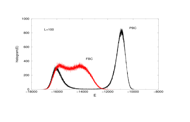
Figure 2: Energy histograms for $L=100$ and $\beta_{MC}^{PBC}=1.342027$ and $\beta_{MC}^{FBC}=1.3378$.

References

- (1) K. Binder and D.W. Heermann Monte Carlo Simulation in Statistical Physics: An Introduction, Springer, Berlin 1988.
- (2) M. Baig, D. Espriu, D.A. Johnston and R.P.K.C. Malmini, J. Phys. A 30, 405 (1997).
- (3) M. Baig, D. Espriu, D.A. Johnston and R.P.K.C. Malmini, J. Phys. A 30, 7695 (1997).
- (4) M. Baig and H. Fort, Phys. Lett. B 332, 428 (1994).
- (5) V. Privman and M.E. Fisher, J. Stat. Phys. 33, 285 (1983).
- (6) K. Binder and D.P. Landau, Phys. Rev. B 30, 1477 (1984).
- (7) M.S.S. Challa, D.P. Landau, and K. Binder, Phys. Rev. B 34, 1841 (1986).
- (8) C. Borgs and R. Kotecký, Journ. Stat. Phys. 61, 79 (1990).
- (9) C. Borgs and R. Kotecký, Journ. Stat. Phys. 79, 43 (1995).
- (10) Medved, diploma Thesis. Charles University. Prague. (http://otokar.troya.nff.cuni.cz/ medved/research/cic.ps)
- (11) K. Binder, Annu. Rev. Phys. Chem. 43, 33 (1992).
- (12) B.V. Enüstün, H.S. Sentürk, and O. Yurdakel, J. Colloid Interface Sci. 65, 509 (1978); S.C. Mraw and D.F. Naas-O’Rourke, Science 205, 901 (1979); J.F. Wendelken and C.-C. Wang, Phys. Rev. B 32, 7542 (1985); V.N. Bogometav, E.V. Kolla, and Yu Kumzerov, JETP Lett. 41, 34 (1985); R. Marx, Phys. Rep. 125, 1 (1985); B.A. Weinstein, Semicond. Sci. Technol. 4, 283 (1989); B. Gorbunov, L.S. Lazareva, A.Z. Gogolev, and E.L. Zhuzhgov, Kolloidn Zh. 51, 921 (1990).
- (13) R.B. Potts, Proc. Camb. Phil. Soc 48, 106 (1952).
- (14) G.K. Saviddy and F.J. Wegner, Nucl. Phys. B 413, 605 (1994).
- (15) J. Clua. ”Efectes Topologics en el Lattice”, PhD. Thesis (UAB) Unpublished. (M. Baig, J. Clua, D.A. Johnston and R. Villanova, in preparation)
- (16) J. Jersak, C.B. Lang and T. Neuhaus, Phys. Rev. D 54, 6909 (1996).
- (17) C. Borgs and R. Kotecký, Phys. Rev. Lett. 68, 1734 (1992).
- (18) C. Borgs, R. Kotecký and S. Miracle-Solé, Journ. Stat. Phys. 62, 529 (1991).
- (19) W. Janke, Phys. Rev. B 47, 14757 (1993).
- (20) F.Y. Wu, Rev. Mod. Phys. 54, 245 (1982).
- (21) A.D. Sokal in Monte Carlo Methods in Statistical Mechanics: Foundations and New Algorithms, lecture notes, Cours de Troisième Cycle de la Physique en Suisse Romande, Lausanne (1989).
- (22) N. Madras and A.D. Sokal, J. Stat. Phys. 50, 109 (1988).
- (23) W. Janke, Monte Carlo Simulations of Spin Systems, in: Computational Physics: Selected Methods – Simple Exercises –Serious Applications, eds. K.H. Hoffmann and M. Schreiber (Springer, Berlin, 1996), p. 10.
- (24) R.G. Miller, Biometrika 61, 1 (1974).
- (25) B. Efron, The Jackknife, the Bootstrap and other Resampling Plans (SIAM, Philadelphia, PA, 1982).
- (26) If this is the case, the phase transition of the 4-d U(1) gauge model with FBC will remain of first order. This point is still under study (M. Baig and R. Villanova, in preparation).
- (27) A.M. Ferrenberg and R.H. Swendsen, Phys. Rev. Lett. 61, 2635 (1988).
- (28) W.H. Press, B.P. Flannery, S.A. Teukolsky, and W.T. Vetterling, Numerical recipes – the art of scientific computing (Cambridge Univ. Press, Cambridge, 1986).
- (29) J. Lee and J.M. Kosterlitz, Phys. Rev. Lett. 65, 137 (1990); Phys. Rev. B 43, 3265 (1991).
- (30) R.J. Baxter, J. Phys. C 6, L445 (1973), using results from his article in J. Stat. Phys. 9, 145 (1973).
- (31) R.J. Baxter, Exactly Solved Models in Statistical Mechanics, Academic Press, London 1982.
- (32) F.Y. Wu and Y.K. Wang, J. Math. Phys. 17, 439 (1976).
- (33) A. Hintermann, H. Kunz, and F.Y. Wu, J. Stat. Phys. 19, 623 (1978).