Abstract

A recently introduced method for determining the critical indices of the deconfinement transition in gauge theories, already tested for the case of 3D SU(3) pure gauge theory, is applied here to 4D SU(2) pure gauge theory. The method is inspired by universality and based on the finite size scaling behavior of the expectation value of simple lattice operators, such as the plaquette. We obtain an accurate determination of the critical index $\nu$, in agreement with the prediction of the Svetitsky-Yaffe conjecture.

1 Introduction

The phase transition from a low temperature phase, where quarks and gluons are confined into hadrons, to a high temperature phase, where a quark-gluon plasma of interacting quasi-particles can appear, is one of the most important features of SU(N) gauge theories at finite temperature. Many present investigations (for a review, see Ref. [1]) are devoted to clarify the kind of phase transition as a function of the number of light quarks and of their masses and to determine the critical temperature. When the phase transition is second order, it becomes essential to determine its critical indices, since they rule the dependence of macroscopic observables on the temperature in the critical region. Moreover, they allow to identify the universality class of the transition and, consequently, the relevant degrees of freedom near criticality.

Pure SU(N) gauge theories at finite temperature possess all essential features of the deconfinement transition and represent an ideal laboratory to understand mechanisms and to set up methods of investigation, since they can be simulated on a space-time lattice with relatively small effort.

The order parameter of the deconfinement transition in a SU(N) pure gauge theory is the Polyakov loop [2, 3], defined as

$$P(\vec{x})\equiv\mbox{Tr}\prod_{n_{4}=1}^{N_{t}}U_{4}(\vec{x},an_{4})\;,$$ (1)

where $U_{\mu}(x)$ is the link variable at the site $x\equiv(\vec{x},t)$ in the $\mu$ direction and $a$ is the lattice spacing. Let us consider the transformation $U_{4}(\vec{x},a\bar{n}_{4})\longrightarrow z\>U_{4}(\vec{x},a\bar{n}_{4})$, where $z$ belongs to the center of the gauge group, Z(N), and $a\bar{n}_{4}$ is any fixed (lattice) time coordinate. Under this transformation the lattice action is left invariant, the Polyakov loop $P(\vec{x})$ transforms instead in $z\>P(\vec{x})$. If the Z(N) symmetry were unbroken, $\langle P\rangle$ should always vanish; instead, owing to spontaneous symmetry breaking, $\langle P\rangle\neq 0$ above a critical temperature $T_{c}$. The deconfinement transition coincides with the spontaneous breaking of the Z(N) global symmetry.

By integrating out all degrees of freedom of the $(d+1)$-dimensional SU(N) gauge theory except the order parameter, it is possible to generate an effective $d$-dimensional statistical model for the Polyakov loop, having Z(N) as global symmetry group. According to the Svetitsky-Yaffe conjecture [4], if the $(d+1)$-dimensional gauge theory undergoes a second order phase transition, its critical indices coincide with those of the effective $d$-dimensional model, if the latter has also a second order phase transition. Moreover their critical behavior, including finite size scaling, is predicted to coincide and is determined essentially by the Z(N) global symmetry. So, in particular, 3D SU(3) pure gauge theory belongs to the universality class of 2D Z(3) (3-state Potts) model and 4D SU(2) pure gauge theory to that of 3D Z(2) (Ising) model.

A new method has recently been proposed [5] (see also [6]) for the computation of the critical indices of a pure gauge theory with second order deconfinement transition. The method, described in detail in the next Section, is based on the finite size behavior of “simple” lattice operators, such as the plaquette, and allows very accurate determinations with small computational effort. It has been already successfully tested for the computation of the critical index $\nu$ of the correlation length for the case of 3D SU(3) pure gauge theory [5]. In that case a precise determination of $\nu$ was obtained, in perfect agreement with the Svetitsky-Yaffe conjecture and with remarkably improved accuracy with respect to an earlier determination based on the Monte Carlo method [7]. Here, we apply the same method to determine $\nu$ for the case of 4D SU(2) pure gauge theory. On the basis of the previous experience [5], we expect to improve the accuracy with respect to the existing determination [8], based on Monte Carlo methods, which gave $\nu_{MC}$=0.630(9).

2 Finite size scaling and the critical index $\nu$

To illustrate the method, let us consider the determination of the critical index $\nu$ of the correlation length $\xi$, defined as

$$\xi\sim|t|^{-\nu}\;,\hskip 85.35826ptt\equiv\frac{T-T_{c}}{T_{c}}\;.$$

For a general $d$-dimensional statistical model a possible way of extracting the value of $\nu$ from lattice Monte Carlo simulations is to study the finite size scaling (FSS) behavior of the energy operator: FSS theory predicts that, if $L$ is the lattice size, the expectation value of the (lattice) energy operator behaves for large $L$ as [9]

$$\langle E\rangle_{L}\sim\langle E\rangle_{\infty}+kL^{\frac{1}{\nu}-d}\;,$$ (2)

where $\langle E\rangle_{\infty}$ is the expectation value of the energy operator in the thermodynamic limit and $k$ is a non-universal constant.

Compared to other methods based on the FSS of fluctuation operators such as susceptibilities or Binder cumulants, the advantage lies in the fact that $\langle E\rangle_{L}$ can be computed to high accuracy. The main drawback is that the term containing $\nu$ in Eq.(2) is subdominant for $L\to\infty$ with respect to the bulk contribution $\langle E\rangle_{\infty}$. The numerical results of Ref. [5] have clearly shown that, in the case of gauge theories, the advantages outweigh the drawbacks and the method can give very accurate results.

In order to apply the same method to the $(d+1)$-dimensional gauge theory, it is necessary to compute expectation values of operators having the same finite size behavior of the energy in the $d$-dimensional statistical model. Let us consider a gauge invariant operator $\hat{O}$ that is invariant also under the global symmetry given by the center of the gauge group, such as any Wilson loop or any correlator of the form

$$P(\vec{x})P^{\dagger}(\vec{y})\;,$$ (3)

where $P(\vec{x})$ and $P(\vec{y})$ are Polyakov loops at two different sites $\vec{x}$ and $\vec{y}$ of the $d$-dimensional space. It is natural to expect that the operator product expansion (OPE) of any such operator at criticality has the same form as the one of $E$:

$$\hat{O}=c_{I}\ I+c_{\epsilon}\ \epsilon+\cdots\;.$$ (4)

Here $I$ and $\epsilon$ are, respectively, the identity and the scaling energy operator in the statistical model, and the dots represent contributions of operators with higher dimension. Two remarks are in order here. First, the scaling energy operator $E$ is not to be confused with the lattice energy operator $E$, which is just an example of an operator in the statistical model with OPE given by Eq. (4). Second, the operators appearing in Eq. (4) are, formally, functionals of the order parameter of the $(d+1)$-dimensional gauge theory, i.e. of the Polyakov loop. The dynamics of the order parameters at criticality is, however, the same in the $(d+1)$-dimensional gauge theory and in the $d$-dimensional statistical model, so that such a distinction is practically unessential.

The ansatz of Eq. (4) was introduced and tested in Ref. [10], and used in Ref. [11, 12], to obtain some exact results on correlation functions of 3D gauge theories at the deconfinement transition.

In particular, Eq. (4) implies that the FSS behavior of the expectation value $\langle\hat{O}\rangle$ will have the form of Eq. (2):

$$\langle\hat{O}\rangle_{L}\sim\langle\hat{O}\rangle_{\infty}+cL^{\frac{1}{\nu}-d}\;.$$ (5)

The contributions of the irrelevant operators will be subleading for $L\to\infty$.

We conclude that the FSS behavior of any such operator can be used to determine the value of $\nu$ through Eq. (5). The obvious advantage is that one can use operators, such as the plaquette, whose expectation value can be computed to high accuracy with relatively modest computational effort.

In the next Section, we use the described method in practice, to determine the critical index $\nu$ for the 4D SU(2) pure gauge theory.

3 Numerical results

The lattice operators we considered are (i) time-like (“electric”) plaquette, (ii) space-like (“magnetic”) plaquette, (iii) the correlator $P(\vec{x})P^{\dagger}(\vec{y})$, with $\vec{x}$ and $\vec{y}$ taken to be nearest neighbors sites in the 3D (spatial) lattice. All these observables possess the required symmetry properties to have an OPE given by Eq. (4), and hence a FSS behavior as in Eq. (5). Moreover they can be computed to high accuracy in Monte Carlo simulations.

Expectation values were computed on lattices with temporal extension $N_{t}=2$ and spatial sizes $L=N_{x}=N_{y}=N_{z}$ ranging from $5$ to $26$. Simulations must be performed at criticality, i.e. at the critical value of the lattice (inverse) coupling constant $\beta$ for the given $N_{t}$. We fixed $\beta$ at the central value of the determination of Ref. [8]: $\beta_{c}(N_{t}=2)$=1.8735. The simulation algorithm we adopted was the over-relaxed heat-bath [13]. For each simulation we collected a number of equilibrium configurations ranging from 50K to 4.8M, according to the lattice size, separated each other by a number of iterations of the order of the autocorrelation time. The error analysis was performed by the jackknife method applied to data bins at different levels of blocking.

We report in Table 1 the expectation values we obtained. Because of the asymmetry of the lattice, space-like and time-like plaquettes have obviously different expectation values and must be considered as two different operators. To evaluate $\nu$, we performed a single multibranched fit of the three data sets. To avoid cross-correlations we included in the fit only magnetic plaquettes from lattices with odd $L$ and electric plaquettes from lattices with even $L$. Polyakov loop correlations were measured in separate runs and therefore are not correlated with the plaquette measurements.

The result of the fit is

$$\nu=0.6298(28)\;,\qquad\qquad\chi^{2}/{\rm d.o.f.}=0.96\;,$$ (6)

in excellent agreement, as predicted by the Svetitsky-Yaffe conjecture, with the most accurate determination for the 3D Ising model, $\nu=0.63012(16)$, obtained in Ref. [14] by the high-temperature expansion method. According to expectations, the accuracy of our result is improved in comparison to the existing Monte Carlo evaluation, based on the $\chi^{2}$ analysis of the topological loop susceptibility, which gives $\nu_{MC}=0.630(9)$ [8].

In Figs. 1-3, we plot the expectation values of electric plaquette, magnetic plaquette and Polyakov loop correlator for different values of $L$ versus $L^{1/\nu-3}$, where $\nu$ is (the central value of) our determination.

4 Conclusions

In this paper, we have applied a recently proposed method for the evaluation of critical indices of the deconfinement transition in pure gauge theories to the case of 4D SU(2). Our result for the critical index $\nu$ of the correlation length confirms the conclusion of the analogous determination for the case of 3D SU(3) by the same method. Namely, the proposed method allows very precise results for critical indices, since it is based on the evaluation of “simple” expectation values, such as that of the plaquette.

The same method can be used to evaluate the critical coupling, which here was taken from the literature: one should perform simulations at different values of $\beta$ in the critical region and, for each of them, determine $\nu$ by the fit with the finite size scaling law; the critical value of $\beta$ can be obtained by comparing the $\chi^{2}$’s of the different fits.

Table 1: Expectation values of electric plaquette, magnetic plaquette and Polyakov loop correlator. Simulations were performed at $\beta=\beta_{c}$=1.8735 on $L^{3}\times 2$ lattices.

$L$	Statistics	Electric plaq.	Magnetic plaq.	$PP$ correlator
5	4800K	0.477152(11)	0.4658468(88)	-
6	2700K	0.475211(11)	0.4652584(87)	-
7	1700K	0.473926(12)	0.4649083(86)	-
7	1100K	-	-	0.40117(14)
8	1200K	0.473002(12)	0.4646322(88)	-
9	800K	0.472354(13)	0.4644188(99)	-
10	600K	0.471832(13)	0.4642710(82)	0.37296(13)
11	450K	0.471449(13)	0.4641638(85)	-
12	350K	0.471127(13)	0.4640621(90)	-
13	280K	0.470850(13)	0.4639818(80)	0.35969(14)
14	280K	0.470659(11)	0.4639314(80)	-
15	200K	0.470482(12)	0.4638766(78)	-
16	150K	0.470290(14)	0.4638078(86)	0.35208(14)
17	120K	0.470169(12)	0.4637843(89)	-
18	100K	0.470065(11)	0.4637625(84)	-
19	90K	0.469948(13)	0.463722(10)	0.34735(15)
20	75K	0.469872(15)	0.4636941(75)	-
21	65K	0.469771(15)	0.4636668(84)	-
22	53K	0.469714(16)	0.4636391(97)	0.34429(23)
23	50K	0.469626(14)	0.4636321(77)	-
24	50K	0.469597(15)	0.4636137(90)	-
25	50K	-	-	0.34165(16)
26	50K	0.469487(15)	0.463571(12)	-

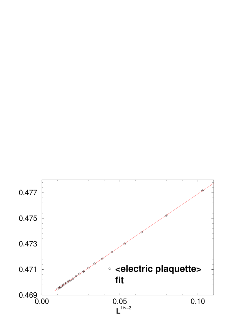
Figure 1: Expectation values of the electric plaquette vs $L^{1/\nu-3}$, with $\nu$ taken as the central value of our determination, i.e. $\nu$=0.6298. Simulations were performed at $\beta=\beta_{c}$=1.8735 on $L^{3}\times 2$ lattices, with $L$ ranging from 5 to 26 (see Table 1).

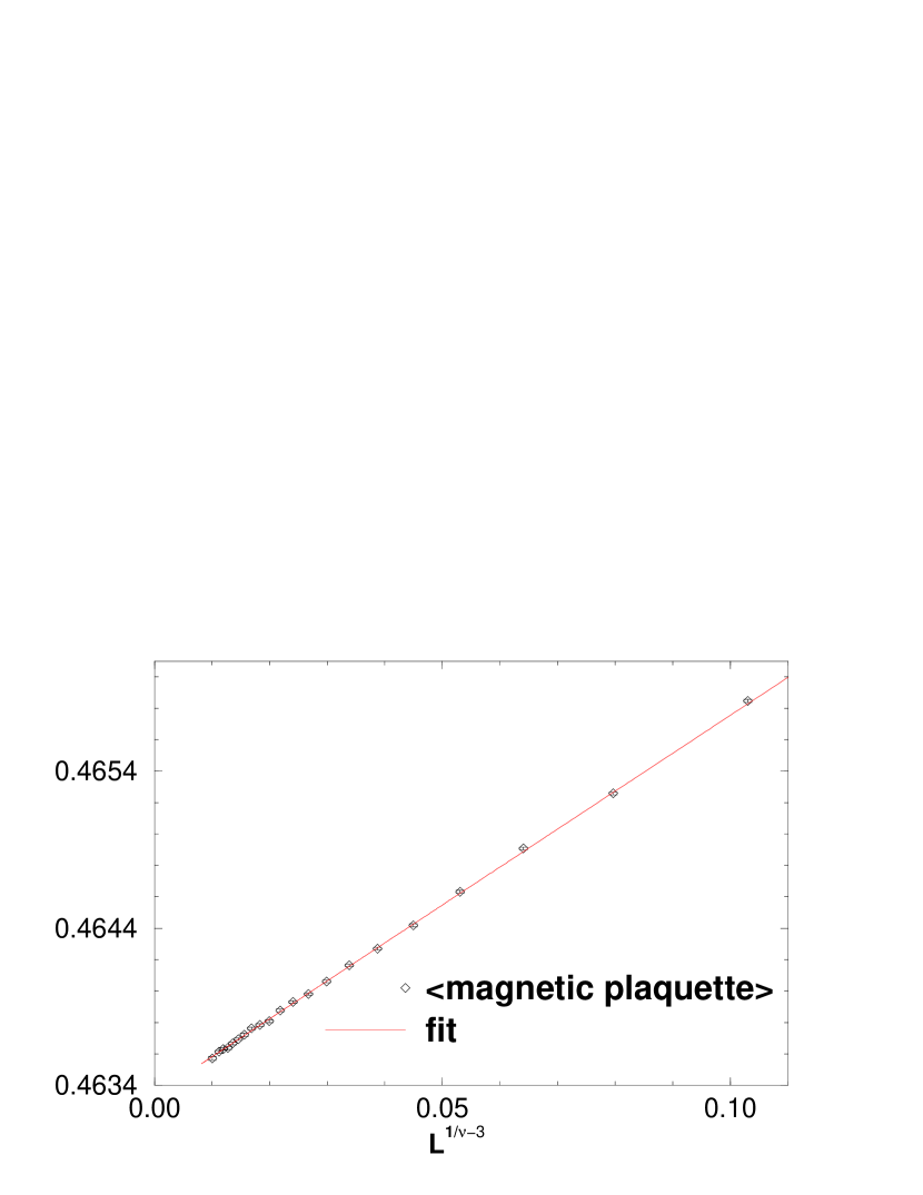
Figure 2: The same as Fig. 1 for the magnetic plaquette.

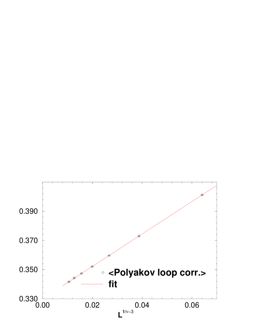
Figure 3: The same as Fig. 1 for the Polyakov loop correlator.

References

- [1] F. Karsch, arXiv:hep-lat/0106019.
- [2] A. M. Polyakov, Phys. Lett. B 72 (1978) 477.
- [3] L. Susskind, Phys. Rev. D 20 (1979) 2610.
- [4] B. Svetitsky and L. G. Yaffe, Nucl. Phys. B 210 (1982) 423.
- [5] R. Fiore, A. Papa and P. Provero, Phys. Rev. D 63 (2001) 117503 [arXiv:hep-lat/0102004].
- [6] R. Fiore, A. Papa and P. Provero, Nucl. Phys. Proc. Suppl. 106 (2002) 486 [arXiv:hep-lat/0110017].
- [7] J. Engels, F. Karsch, E. Laermann, C. Legeland, M. Lutgemeier, B. Petersson and T. Scheideler, Nucl. Phys. Proc. Suppl. 53 (1997) 420 [arXiv:hep-lat/9608099].
- [8] S. Fortunato, F. Karsch, P. Petreczky and H. Satz, Nucl. Phys. Proc. Suppl. 94 (2001) 398 [arXiv:hep-lat/0010026].
- [9] M. Hasenbusch and K. Pinn, J. Phys. A 31 (1998) 6157 [arXiv:cond-mat/9706003].
- [10] F. Gliozzi and P. Provero, Phys. Rev. D 56 (1997) 1131 [arXiv:hep-lat/9701014].
- [11] R. Fiore, F. Gliozzi and P. Provero, Phys. Rev. D 58 (1998) 114502 [arXiv:hep-lat/9806017].
- [12] R. Fiore, F. Gliozzi and P. Provero, Nucl. Phys. Proc. Suppl. 73 (1999) 429 [arXiv:hep-lat/9807037].
- [13] R. Petronzio and E. Vicari, Phys. Lett. B 254 (1991) 444.
- [14] M. Campostrini, A. Pelissetto, P. Rossi and E. Vicari, arXiv:cond-mat/0201180.