Lattice quark propagator with staggered quarks in Landau and Laplacian gauges
Abstract
We report on the lattice quark propagator using standard and improved Staggered quark actions, with the standard, Wilson gauge action. The standard Kogut-Susskind action has errors of while the “Asqtad” action has , errors. The quark propagator is interesting for studying the phenomenon of dynamical chiral symmetry breaking and as a test-bed for improvement. Gauge dependent quantities from lattice simulations may be affected by Gribov copies. We explore this by studying the quark propagator in both Landau and Laplacian gauges. Landau and Laplacian gauges are found to produce very similar results for the quark propagator.
I Introduction
The quark propagator lies at the heart of most QCD physics. In the low momentum region it exhibits dynamical chiral symmetry breaking (which cannot be seen from perturbation theory) and at high momentum can be used to extract the running quark mass Aok99 ; Bec00b (which cannot be extracted directly from experiment). In lattice QCD, quark propagators are tied together to extract hadron masses. Lattice gauge theory provides a way to study the quark propagator nonperturbatively, possibly as a way of calculating the chiral condensate and , and in turn, such a study can provide technical insight into lattice gauge theory.
We study the quark propagator using the Kogut-Susskind (KS) fermion action, which has errors, and an improved staggered action, Asqtad Org99 , which has errors of , . These choices complement other studies using Clover Sku01a ; Sku01b and Overlap overlap quarks. We are required to gauge fix and we choose the ever popular Landau gauge and the interesting Laplacian gauge Vin92 ; Vin95 . Laplacian gauge fixing is an unambiguous gauge fixing and, although it is difficult to understand perturbatively, it is equivalent to Landau gauge in the asymptotic region. It has been used to study the gluon propagator Ale01 ; Ale02 ; lapglu .
In there are various ways to implement a Laplacian gauge fixing. Three varieties of Laplacian gauge fixing are used, and these form three different, but related gauges. This is briefly discussed in section III. For a more detailed discussion, see Ref. lapglu .
The quark propagator was calculated on 80, configurations generated with the standard Wilson gluon action at ( fm)111Some of numbers in this report differ slightly from those published elsewhere proc_quark01 due to a revised value for the lattice spacing.. We have used six quark masses: , 0.0625, 0.05, 0.0375, 0.025 and 0.0125 (114 to 19 MeV).
II Lattice Quark Propagator
In the continuum, Lorentz invariance allows us to decompose the full propagator into Dirac vector and scalar pieces
| (1) |
or, alternatively,
| (2) |
This is the bare propagator which, once regularized, is related to the renormalized propagator through the renormalization constant
| (3) |
where is some regularization parameter, e.g. lattice spacing. Asymptotic freedom implies that, as , reduces to the free propagator
| (4) |
where is the bare quark mass.
The tadpole improved, tree-level form of the KS quark propagator is
| (5) |
where is the discrete lattice momentum given by
| (6) |
For the tadpole factor, we employ the plaquette measure,
| (7) |
We give a detailed discussion of the notation used for the staggered quark actions in an appendix. As a convienient short-hand we define a new momentum variable for the KS quark propagator,
| (8) |
We can then decompose the inverse propagator222This is intended to be merely illustrative; in practice we never actually invert the propagator. See appendix for details.
| (9) | |||
| (10) |
where the factor of 16 comes from the trace over the spin-flavor indices of the staggered quarks and from the trace over color. Comparing Eqs. (4) and (5) we see that dividing out in Eq. (9) is analagous to dividing out in the continuum and ensures that that has the correct asymptotic behavior. So by considering the propagator as a function of , we ensure that the lattice quark propagator has the correct tree-level form, i.e.,
| (11) |
and hopefully better approximates its continuum behavior. This is the same philosophy that has been used in studies of the gluon propagator gluon and Eq. (8) was used to define the momentum in Ref. Bec00b .
The Asqtad quark action Org99 is a fat-link Staggered action using three-link, five-link and seven-link staples to minimize flavor changing interactions along with the three-link Naik term Nai89 (to correct the dispersion relation) and planar five-link Lepage term Lep99 (to correct the IR). The coefficients are tadpole improved and tuned to remove all tree-level errors. This action was motivated by the desire to improve flavor symmetry, but has also been reported to have good rotational properties.
The quark propagator with this action has the tree-level form
| (12) |
so we repeat the above analysis, this time defining
| (13) |
Finally, it should be noted that both actions get contributions from tadpoles, which can be seen in the tree-level behaviors of the two invariants
| (14) | ||||
| (15) |
so inserting the tadpole factors provides the correct normalization.
III Gauge Fixing
We consider the quark propagator in Landau and Laplacian gauges. Landau gauge fixing is performed by enforcing the Lorentz gauge condition, on a configuration by configuration basis. This is achieved by maximizing the functional,
| (16) |
by, in this case, a Fourier accelerated, steepest-descents algorithm Dav88 . There are, in general, many such maxima and these are called lattice Gribov copies. While this ambiguity has produced no identified artefacts in QCD, in principle it remains a source of uncontrolled systematic error.
Laplacian gauge is a nonlinear gauge fixing that respects rotational invariance, has been seen to be smooth, yet is free of Gribov ambiguity. It is also computationally cheaper then Landau gauge. There is, however, more than one way of obtaining such a gauge fixing in . The three implementations of Laplacian gauge fixing employed here are (in our notation):
-
1.
(I) gauge (QR decomposition), used by Alexandrou et al. Ale01 .
-
2.
(II) gauge, where the Laplacian gauge transformation is projected onto by maximising its trace lapglu .
- 3.
All three versions reduce to the same gauge in SU(2). For a more detailed discussion, see Ref. lapglu .
IV Analysis of Lattice Artefacts
IV.1 Tree-level Correction
As mentioned above, the idea of “kinematic” or “tree-level” correction has been used widely in studies of the gluon propagator gluon and the quark propagator Sku01a ; Sku01b ; overlap and we investigate its application to our quark propagators. For the moment we shall restrict ourselves to Landau gauge. To help us understand the lattice artefacts, we separate the data into momenta lying entirely on a spatial cartesian direction (squares), along the temporal direction (triangles), the four-diagonal (diamonds) or some other combination of directions (circles).
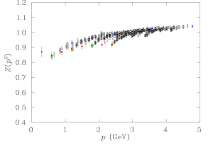
The function is plotted for the KS action in Fig. 1, comparing the results using and . In the top of Fig. 1 we see substantial hypercubic artefacts (in particular look at the difference between the diamond and the triangle at around 2.5 GeV). We can suggest that this is caused by violation of rotational symmetry because the agreement between triangles and squares suggests that finite volume effects are small in the region of interest. In the plot below, where has been used, we see some restoration of rotational symmetry.
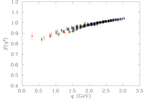
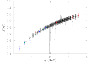
The same study is made for the Asqtad action in Fig. 2. In both cases this action shows a substantial improvement over the KS action, and when we plot using , the momentum defined by the action, rotational asymmetry is reduced to the level of the statistical errors.
It is less clear which momentum variable should be used for the mass function, so for consistency we use , as for the function. The effect of this is shown in Fig. 3. For ease of comparison, both sets of data have been cylinder cut gluon . In the case of the mass function, the choice of momentum will actually make little difference to our results.
IV.2 Comparison of the actions
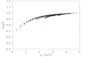
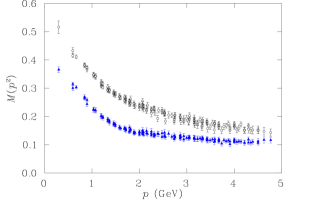
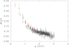
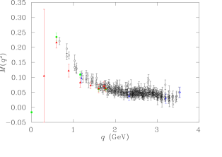
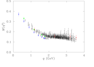
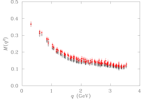
In Fig. 4 the mass function is plotted, in Landau gauge, for both actions with quark mass . This time there have been no data cuts. We see that the KS action gives a much larger value for M(0) than the Asqtad action and is slower to approach asymptotic behavior. Asqtad also shows slightly better rotational symmetry.
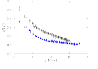
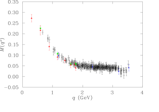
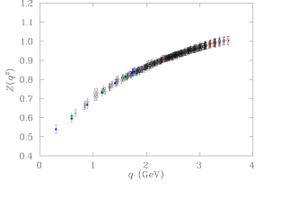
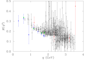
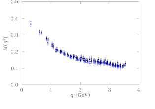
Looking back at Figs. 1 and 2 we see that the Asqtad action displays clearly better rotational symmetry in the quark function and, curiously, improved infrared behavior as well. The Asqtad action also displays a better approach to asymptotic behavior, approaching one in the ultraviolet. The relative improvement increases as the quark mass decreases. In Fig. 5 we compare the mass function for the two actions at , the lowest mass studied here. The low quark mass has introduced less noise into the propagator with the Asqtad action than with the KS action.
IV.3 Comparitive performance of Landau and Laplacian gauges
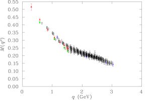
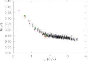
Fig. 6 shows the mass function for the Asqtad action in (I) and (II) gauges and it should be compared with the equivalent Landau gauge result in Fig. 4. We see firstly that these three gauges give very similar results (we shall investigate this in more detail later) and secondly that they give similar performance in terms of rotational symmetry and statistical noise. Looking more closely, we can see that the Landau gauge gives a slightly cleaner signal at this lattice spacing.
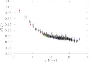
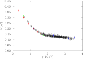
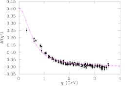
Landau gauge seems to respond somewhat better than (II) gauge to vanishing quark mass; compare Fig. 7 with Fig. 5. In Fig. 7 we see large errors in the infrared region and points along the temporal axis lying below the bulk of the data. These are indicators of finite volume effects, an unexpected result given that earlier gluon propagator studies Ale01 ; Ale02 appear to conclude that Laplacian gauge is less sensitive to volume than Landau gauge.
(III) performs very poorly: see Figs. 8 and 9. The gauge fixing procedure failed for four of the configurations and eight of the remaining configurations produced and M functions with pathological negative values. We have seen that this type of gauge fixing fails to produce a gluon propagator that has the correct asymptotic behavior lapglu . It seems likely that we are dealing with matrices with vanishing determinants, which are destroying the projection onto . We expect the degree to which this problem occurs to be dependent on the simulation parameters and the numerical precision used (in this work the gauge transformations were calculated in single precision).
V Gauge Dependence
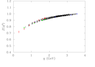
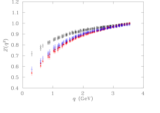
Now we investigate the quark mass and functions in Landau, (I) and (II) gauges. Fig. 10 shows the function for the Asqtad action in Landau and (I) gauges. They are in excellent agreement in the ultraviolet - as they ought - but differ significantly in the infrared. The function in the Laplacian gauges is more strongly infrared suppressed than in the Landau gauge. There may be a small difference in between (I) and (II) gauges.
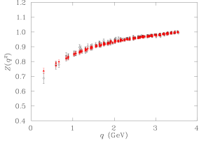
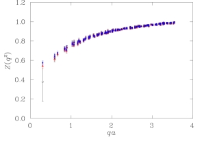
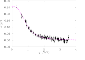
In all cases the quark function demonstrates little mass dependence. Deviation of from its asymptotic value of 1 is a sign of dynamical symmetry breaking, so we expect the infrared suppression to go away in the limit of an infinitely heavy quark. In Fig. 11 we show the function in Landau gauge for the lightest and the heaviest quark masses in this study. The two are the same, to within errors, although if we look at the lowest momentum data we see that the point for the low mass lies below the high mass one. Fig. 12 shows in (II) gauge for three quark masses. Again, the data are consistent, to within errors, but there is a systematic ordering of lightest to heaviest. We conclude from this that behavior is consistent with expectations, dependence on the quark mass - if any - is very weak. One possible explanation is that all the masses studied are light - less than or approximately equal to the stange quark mass - and that heavier masses will affect the function more clearly.
The mass functions in Landau and (I) gauges - shown in Fig. 13 - agree to within errors. The data for (I) gauge seems to sit a little higher than the Landau gauge through most of the momentum range, so with greater statistics we may resolve a small difference. The mass functions are nearly identical in (I) and (II) gauges: see Fig. 14.
VI Modelling the Mass function
The Asqtad quark mass function at each value of the mass has been cylinder cut and extrapolated - by a quadratic fit - to zero mass. The quadratic fit was chosen on purely practical grounds and a linear fit worked almost as well. A fit to each of the mass functions was then done, using the ansatz
| (17) |
which is a generalization of the one used in Ref. Sku01a . As we have seen, the quark mass function in the Laplacian gauge is almost indistinguishable from that in the Landau gauge, except that it is somewhat noisier (this may change at smaller lattice spacing). For this reason, we only show fits in the Landau gauge. Table I shows a sample of the fits. The table is divided into two sections, one in which the parameter was held fixed, one in which it was allowed to vary. We see that for the heaviest mass, provides an excellent fit, but in the chiral limit, is somewhat favored. The rôle of may be seen if Fig. 15. At , the infrared and ultraviolet are significantly flatter, while the mass generation at around one GeV is made steeper.
| c | ||||||
| (MeV) | (MeV) | (MeV) | (MeV) | per d.o.f. | ||
| 114 | 0.35(1) | 910(20) | 142(7) | 1.0 | 462(9) | 0.38 |
| 95 | 0.36(5) | 880(70) | 117(7) | 1.0 | 440(20) | 0.42 |
| 76 | 0.39(5) | 830(70) | 92(7) | 1.0 | 420(20) | 0.42 |
| 57 | 0.45(4) | 770(50) | 70(7) | 1.0 | 410(20) | 0.51 |
| 38 | 0.49(8) | 720(60) | 44(6) | 1.0 | 400(30) | 0.56 |
| 19 | 0.54(9) | 670(60) | 18(6) | 1.0 | 380(30) | 0.69 |
| 0 | 0.56(8) | 650(50) | -12(6) | 1.0 | 350(20) | 0.66 |
| 0 | 0.80(20) | 520(50) | 0.0 | 1.0 | 400(40) | 1.3 |
| 114 | 0.28(1) | 990(30) | 155(7) | 1.25(4) | 428(7) | 0.38 |
| 95 | 0.28(2) | 965(40) | 129(9) | 1.30(10) | 404(9) | 0.37 |
| 76 | 0.30(2) | 930(50) | 105(7) | 1.29(6) | 380(10) | 0.36 |
| 57 | 0.30(2) | 910(40) | 80(6) | 1.30(2) | 354(9) | 0.41 |
| 38 | 0.36(4) | 830(50) | 54(7) | 1.28(7) | 350(20) | 0.46 |
| 19 | 0.30(10) | 800(200) | 29(6) | 1.4(3) | 310(60) | 0.55 |
| 0 | 0.30(4) | 870(60) | 0.0 | 1.52(23) | 260(20) | 0.49 |
In this model, is acting as a function of the bare mass, controlling the dynamical symmetry breaking. Unfortunately, the paucity of data points in the infrared leaves poorly determined in the chiral limit. Furthermore, the degree to which our infrared data may be affected by the finite volume and by the chiral extrapolation is not really known. Finally, this ansatz is still crude in that it does not provide the correct asymptotic behavior.
As was explained is Section II, the quark mass function approaches the renormalised quark mass in the ultraviolet, which itself becomes the bare mass in the limit. It is a general feature of this study that the ultraviolet tail of sits somewhat higher than the bare mass. The situation is summarised in Table 2. This deviation from the correct asymptotic behavior is probably the consequence of an insufficiently small lattice spacing.
| (MeV) | M(0) (MeV) | M(0) (MeV) | ||
|---|---|---|---|---|
| 114 | 462(9) | 1.25(6) | 428(7) | 1.35(6) |
| 95 | 440(20) | 1.23(7) | 404(9) | 1.36(6) |
| 76 | 420(20) | 1.21(9) | 380(10) | 1.38(9) |
| 57 | 410(20) | 1.2(1) | 354(9) | 1.4(1) |
| 38 | 400(30) | 1.16(16) | 350(20) | 1.4(2) |
| 19 | 380(30) | 1.0(3) | 310(60) | 1.5(3) |
VII Conclusions
We have seen that the Asqtad action provides a quark propagtor with improved rotational symmetry compared to the standard Kogut-Susskind action and that the difference between them increases as we go to lighter quark masses. Furthermore, we have seen that the Asqtad action has smaller mass renormalization and better asymptotic behavior.
Our results for the quark propagator show that the quark mass function is the same, to within statistics in (I) and (II) gauges, while the function is slightly different. There is little difference between the quark mass function in Landau gauge and in Laplacian gauge, but the function dips more strongly in the infrared in Laplacian gauge than in Landau gauge. The infrared region of the Laplacian gauge mass function seems to be particularly badly affected by decreasing quark mass. We have seen that the (III) gauge gives very poor results in , in calculations of the quark propagator, consistent with results for the gluon propagator lapglu . Overall the Landau gauge results of this work for the Asqtad appear to be consistent within errors with the results of ealier Landau gauge studies of the quark propagator [4,5,6]. Our results suggest that the function is insensitive to whether we use Landau or Laplacian gauge, whereas the function has an enhanced infrared dip in Laplacian gauge.
As we have simulated on only one lattice, it remains to do a thorough examination of discretization and finite volume effects. The chiral limit was obtained by extrapolation, which may provide another source of systematic error. It will also be interesting to investigate the errors by using an improved gluon action. Further work may allow the development of a more sophisticated ansatz which has the correct asymptotic behavior. Finally, studies on finer lattices could be used to calculate the chiral condensate, light quark masses and potentially .
Acknowledgements.
The authors wish to thank Derek Leinweber and Jonivar Skullerud for useful discussions. The work of UMH and POB was supported in part by DOE contract DE-FG02-97ER41022. The work of AGW was supported by the Australian Research Council.*
Appendix A Staggered quark propagators
In this appendix we give details of the quark propagator calculation using the Kogut-Susskind and Asqtad actions. The free KS action is
| (18) |
where the staggered phases are: and
| (19) |
To Fourier transform, write
| (20) |
as , where
| (21) | |||
| (22) |
and define . Then
| (23) | |||
| (24) |
Defining
| (25) | ||||
| (26) |
where the satisfy
| (27) | |||
| (28) |
forming a “staggered” Dirac algebra. Putting all this together, we can derive a momentum space expression for the KS action,
| (29) |
From this we can see that, in momentum space, the tadpole improved, tree-level form of the quark propagator is
| (30) |
where is the discrete lattice momentum given by Eq. (21). Assuming that the full propagator retains this form (in analogy to the continuum case) we write
| (31) | ||||
| (32) |
For the KS action, it is convenient to define
| (33) |
as a shorthand.
Numerically, we calculate the quark propagator in coordinate space,
| (34) |
To obtain the quark propagator in momentum space, we take the Fourier transform of and, decomposing the momenta as , get
| (35) |
Thus, in terms of the KS momenta, ,
| (36) |
from which we obtain
| (37) |
and
| (38) |
Note: we could determine
| (39) | ||||
| (40) |
but we would rather avoid inverting .
Putting it all together we get
| (41) | ||||
| (42) | ||||
| (43) |
The tadpole improved, tree-level behavior of the and mass functions are simply
| (44) |
and
| (45) |
respectively.
The Asqtad quark action Org99 is a fat-link Staggered action using three-link, five-link and seven-link staples along with the three-link Naik term Nai89 and five-link Lepage term Lep99 , with tadpole improved coefficients tuned to remove all tree-level errors. This action was motivated by the desire to minimize quark flavour changing interactions, but has also been reported to have good rotational symmetry.
At tree-level (i.e. no interations, links set to the identity), the staples in this action make no contribution, so the action reduces to the Naik action.
| (46) |
The quark propagator with this action has the tree-level form
| (47) |
so we choose
| (48) | ||||
| (49) |
Having identified the correct momentum for this action, we can calculate the invariant functions as before. No further tree-level correction is required.
References
- (1) S. Aoki et al., Phys. Rev. Lett. 82, 4392 (1999).
- (2) D. Becirevic et al., Phys. Rev. D 61, 114507 (2000).
- (3) K. Orginos, D. Toussaint and R.L. Sugar, Phys. Rev. D 60, 054503 (1999).
- (4) J-I. Skullerud and A.G. Williams, Phys. Rev. D 63, 054508 (2001).
- (5) J-I. Skullerud, D.B. Leinweber and A.G. Williams, Phys. Rev. D 64, 074508 (2001).
- (6) F.D.R. Bonnet, P.O. Bowman, D.B. Leinweber, A.G. Williams and J. Zhang, hep-lat/0202003.
- (7) J.C. Vink and U-J. Wiese, Phys. Lett. B 289, 122 (1992).
- (8) J.C. Vink, Phys. Rev. D 51, 1292 (1995).
- (9) C. Alexandrou, Ph. de Forcrand and E. Follana, Phys. Rev. D 63, 094504 (2001).
- (10) C. Alexandrou, Ph. de Forcrand and E. Follana, hep-lat/0112043.
- (11) P.O. Bowman, U.M. Heller, D.B. Leinweber and A.G. Williams, In preparation.
- (12) F.D.R. Bonnet, P.O. Bowman, D.B. Leinweber, A.G. Williams and J.M. Zanotti, Phys. Rev. D 64, 034501 (2001) and references contained therein.
- (13) S. Naik, Nucl. Phys. B 316, 238 (1989).
- (14) G.P. Lepage, Phys. Rev. D 59, 074502 (1999).
- (15) C.T.H. Davies et al., Phys. Rev. D 37, 1581 (1988).
- (16) P.O. Bowman, U.M. Heller and A.G. Williams, Nucl. Phys. B (Proc. Suppl.) 106, 820 (2002); P.O. Bowman, U.M. Heller and A.G. Williams, hep-lat/0112027.