Excited Baryons in Lattice QCD

Abstract

We present first results for the masses of positive and negative parity excited baryons calculated in lattice QCD using an ${\cal O}(a^{2})$-improved gluon action and a fat-link irrelevant clover (FLIC) fermion action in which only the irrelevant operators are constructed with APE-smeared links. The results are in agreement with earlier calculations of $N^{*}$ resonances using improved actions and exhibit a clear mass splitting between the nucleon and its chiral partner. An correlation matrix analysis reveals two low-lying $J^{P}={1\over 2}^{-}$ states with a small mass splitting. The study of different $\Lambda$ interpolating fields suggests a similar splitting between the lowest two $\Lambda\frac{1}{2}^{-}$ octet states. However, the empirical mass suppression of the $\Lambda^{*}(1405)$ is not evident in these quenched QCD simulations, suggesting a potentially important role for the meson cloud of the $\Lambda^{*}(1405)$ and/or a need for more exotic interpolating fields.

I Introduction

Understanding the dynamics responsible for baryon excitations provides valuable insight into the forces which confine quarks inside baryons and into the nature of QCD in the nonperturbative regime. This is a driving force behind the experimental effort of the CLAS Collaboration at Jefferson Lab, which is currently accumulating data of unprecedented quality and quantity on various $N\to N^{*}$ transitions. With the increased precision of the data comes a growing need to understand the observed $N^{*}$ spectrum within QCD. Although phenomenological low-energy models of QCD have been successful in describing many features of the $N^{*}$ spectrum (for a recent review see Ref. CR ), they leave many questions unanswered, and calculations of $N^{*}$ properties from first principles are indispensable.

One of the long-standing puzzles in spectroscopy has been the low mass of the first positive parity excitation of the nucleon (the $J^{P}={1\over 2}^{+}$ $N^{*}(1440)$ Roper resonance) compared with the lowest lying odd parity excitation. In a valence quark model, in a harmonic oscillator basis, the ${1\over 2}^{-}$ state naturally occurs below the $N=2$, ${1\over 2}^{+}$ state IK . Without fine tuning of parameters, valence quark models tend to leave the mass of the Roper resonance too high. Similar difficulties in the level orderings appear for the ${3\over 2}^{+}$ $\Delta^{*}(1600)$ and ${1\over 2}^{+}$ $\Sigma^{*}(1690)$, which has led to speculations that the Roper resonances may be more appropriately viewed as “breathing modes” of the states BREATHE , or described in terms of meson-baryon dynamics alone FZJ , or as hybrid baryon states with explicitly excited glue field configurations LBL .

Another challenge for spectroscopy is presented by the $\Lambda^{1/2-}(1405)$, whose anomalously small mass has been interpreted as an indication of strong coupled channel effects involving $\Sigma\pi$, $\bar{K}N$, $\ldots$ L1405 , and a weak overlap with a three-valence constituent-quark state. In fact, the role played by Goldstone bosons in baryon spectroscopy has received considerable attention recently MASSEXTR ; YOUNG .

It has been argued GBE that a spin-flavour interaction associated with the exchange of a pseudoscalar nonet of Goldstone bosons between quarks can better explain the level orderings and hyperfine mass splittings than the traditional (colour-magnetic) one gluon exchange mechanism. On the other hand, some elements of this approach, such as the generalisation to the meson sector or consistency with the chiral properties of QCD, remain controversial CR ; ISGUR ; TK . Furthermore, neither spin-flavour nor colour-magnetic interactions are able to account for the mass splitting between the $\Lambda^{1/2^{-}}(1405)$ and the $\Lambda^{3/2^{-}}(1520)$ (a splitting between these can arise in constituent quark models with a spin-orbit interaction, however, this is known to lead to spurious mass splittings elsewhere CR ; CI ). Recent work LARGE_NC on negative parity baryon spectroscopy in the large-$N_{c}$ limit has identified important operators associated with spin-spin, spin-flavour and other interactions which go beyond the simple constituent quark model, as anticipated by early QCD sum-rule analyses Leinweber:hh .

The large number of states predicted by the constituent quark model and its generalisations which have not been observed (the so-called “missing” resonances) presents another problem for spectroscopy. If these states do not exist, this may suggest that perhaps a quark–diquark picture (with fewer degrees of freedom) could afford a more efficient description, although lattice simulation results provide no evidence for diquark clustering DIQ . On the other hand, the missing states could simply have weak couplings to the $\pi N$ system CR . Such a situation would present lattice QCD with a unique opportunity to complement experimental searches for $N^{*}$’s, by identifying excited states not easily accessible to experiment (as in the case of glueballs or hybrids).

In attempting to answer these questions, one fact that will be clear is that it is not sufficient to look only at the standard low mass hadrons ($\pi,\rho,N$ and $\Delta$) on the lattice — one must consider the entire $N^{*}$ (and in fact the entire excited baryon) spectrum. In this paper we present the first results of octet baryon mass simulations using an ${\cal O}(a^{2})$ improved gluon action and an improved Fat Link Irrelevant Clover (FLIC) FATJAMES quark action in which only the irrelevant operators are constructed using fat links FATLINK . Configurations are generated on the Orion supercomputer at the University of Adelaide. After reviewing in Section II the main elements of lattice calculations of excited hadron masses and a brief overview of earlier calculations, we describe in Section III various features of interpolating fields used in this analysis. Section IV reviews the details of the lattice simulations, and Section V gives an overview of the methodology for isolating baryon resonance properties. In Section VI we present the results from our simulations and in Section VII make concluding remarks and discuss possible future extensions of this work.

II Excited Baryons on the Lattice

The history of excited baryons on the lattice is quite brief, although recently there has been growing interest in finding new techniques to isolate excited baryons, motivated partly by the experimental $N^{*}$ program at Jefferson Lab. The first detailed analysis of the positive parity excitation of the nucleon was performed by Leinweber LEIN1 using Wilson fermions and an operator product expansion spectral ansatz. DeGrand and Hecht DEGRAND92 used a wave function ansatz to access $P$-wave baryons, with Wilson fermions and relatively heavy quarks. Subsequently, Lee and Leinweber LL introduced a parity projection technique to study the negative parity ${1\over 2}^{-}$ states using an ${\cal O}(a^{2})$ tree-level tadpole-improved D_χ34 quark action, and an ${\cal O}(a^{2})$ tree-level tadpole-improved gauge action. Following this, Lee LEE reported results using a D₂₃₄ quark action with an improved gauge action on an anisotropic lattice to study the ${1\over 2}^{+}$ and ${1\over 2}^{-}$ excitations of the nucleon. The RIKEN-BNL group DWF has also performed an analysis of the $N^{*}({1\over 2}^{-})$ and $N^{\prime}({1\over 2}^{+})$ excited states using domain wall fermions. More recently, a nonperturbatively improved clover quark action has been used by Richards et al. RICHARDS to study the $N^{*}({1\over 2}^{-})$ and $\Delta^{*}({3\over 2}^{-})$ states, while Nakajima et al. have studied the $N^{*}({1\over 2}^{-})$ and $\Lambda^{*}({1\over 2}^{-})$ states using an anisotropic lattice with an ${\cal O}(a)$ improved quark action Nakajima:2001js . Constrained-fitting methods based on Bayesian priors have also recently been used by Lee et al. BAYESIAN to study the two lowest octet and decuplet positive and negative parity baryons using overlap fermions with pion masses down to $\sim 180$ MeV. While these authors claim to have observed the Roper in quenched QCD, it remains to be demonstrated that this conclusion is independent of the Bayesian-prior assumed in their analysisLEIN1 ; ALLTON .

Following standard notation, we define a two-point correlation function for a spin-$\frac{1}{2}$ baryon $B$ as

$$G_{B}(t,{\vec{p}})\equiv\sum_{\vec{x}}\,e^{-i{\vec{p}}\cdot{\vec{x}}}\left\langle\Omega\left|\chi_{B}(x)\bar{\chi}_{B}(0)\right|\Omega\right\rangle$$ (1)

where $\chi_{B}$ is a baryon interpolating field and where we have suppressed Dirac indices. All formalism for correlation functions and interpolating fields presented in this paper is carried out using the Dirac representation of the $\gamma$-matrices. The choice of interpolating field $\chi_{B}$ is discussed in Section III below. The overlap of the interpolating field $\chi_{B}$ with positive or negative parity states $|B^{\pm}\rangle$ is parameterised by a coupling strength $\lambda_{B^{\pm}}$ which is complex in general and which is defined by

$$\left\langle\Omega\left|\,\chi_{B}(0)\,\right|B^{+},p,s\right\rangle\!\! = \!\!\lambda_{B^{+}}\sqrt{M_{B^{+}}\over E_{B^{+}}}\ u_{B^{+}}(p,s)\,,$$ (2a)

$$\left\langle\Omega\left|\,\chi_{B}(0)\,\right|B^{-},p,s\right\rangle\!\! = \!\!\lambda_{B^{-}}\sqrt{M_{B^{-}}\over E_{B^{-}}}\,\gamma_{5}u_{B^{-}}(p,s)\,,$$ (2b)

where $M_{B^{\pm}}$ is the mass of the state $B^{\pm}$, $E_{B^{\pm}}=\sqrt{M_{B^{\pm}}^{2}+{\vec{p}\,}^{2}}$ is its energy, and $u_{B^{\pm}}(p,s)$ is a Dirac spinor with normalisation $\overline{u}_{B^{\pm}}^{\alpha}(p,s)u_{B^{\pm}}^{\beta}(p,s)=\delta^{\alpha\beta}$. For large Euclidean time, the correlation function can be written as a sum of the lowest energy positive and negative parity contributions

$$G_{B}(t,{\vec{p}}) \approx \lambda_{B^{+}}^{2}{\left(\gamma\cdot p+M_{B^{+}}\right)\over 2E_{B^{+}}}e^{-E_{B^{+}}\,t}$$ (3)

$$+ \lambda_{B^{-}}^{2}{\left(\gamma\cdot p-M_{B^{-}}\right)\over 2E_{B^{-}}}e^{-E_{B^{-}}\,t}\ ,$$

when a fixed boundary condition in the time direction is used to remove backward propagating states. The positive and negative parity states are isolated by taking the trace of $G_{B}$ with the operator $\Gamma_{+}$ and $\Gamma_{-}$ respectively, where

$$\Gamma_{\pm} = {1\over 2}\left(1\pm{M_{B^{\mp}}\over E_{B^{\mp}}}\gamma_{4}\right)\ .$$ (4)

For $\vec{p}=0$, $\Gamma_{\pm}^{2}=\Gamma_{\pm}$ so that $\Gamma_{\pm}$ are then parity projectors. For $\vec{p}=0$, the energy $E_{B^{\pm}}=M_{B^{\pm}}$ and using the operator $\Gamma_{\pm}$ we can isolate the mass of the baryon $B^{\pm}$. In this case, positive parity states propagate in the (1, 1) and (2, 2) elements of the Dirac matrix of Eq. (3), while negative parity states propagate in the (3, 3) and (4, 4) elements.

In terms of the correlation function $G_{B}$, the baryon effective mass function is defined by

$$M_{B}(t)=\log[G_{B}(t,\vec{0})]-\log[G_{B}(t+1,\vec{0})]\ .$$ (5)

Meson masses are determined via analogous standard procedures.

III Interpolating Fields

In this analysis we consider two types of interpolating fields which have been used in the literature. The notation adopted is similar to that of Ref. LWD . To access the positive parity proton we use as interpolating fields

$$\chi_{1}^{p+}(x) = \epsilon_{abc}\left(u^{T}_{a}(x)\ C\gamma_{5}\ d_{b}(x)\right)u_{c}(x)\ ,$$ (6)

and

$$\chi_{2}^{p+}(x) = \epsilon_{abc}\left(u^{T}_{a}(x)\ C\ d_{b}(x)\right)\gamma_{5}\ u_{c}(x)\ ,$$ (7)

where the fields $u$, $d$ are evaluated at Euclidean space-time point $x$, $C$ is the charge conjugation matrix, $a,b$ and $c$ are colour labels, and the superscript $T$ denotes the transpose. These interpolating fields transform as a spinor under a parity transformation. That is, if the quark fields $q_{a}(x)\ (q=u,d,\cdots)$ transform as

$${\cal P}q_{a}(x){\cal P}^{\dagger}=+\gamma_{0}q_{a}(\tilde{x})\ ,$$

where $\tilde{x}=(x_{0},-\vec{x})$, then

$${\cal P}\chi^{p+}(x){\cal P}^{\dagger}=+\gamma_{0}\chi^{p+}(\tilde{x})\ .$$

For convenience, we introduce the shorthand notation

$${\cal G}(S_{f_{1}},S_{f_{2}},S_{f_{3}})\equiv\epsilon^{abc}\epsilon^{a^{\prime}b^{\prime}c^{\prime}}\biggl{\{}S_{f_{1}}^{aa^{\prime}}(x,0)\,{\rm tr}\left[S_{f_{2}}^{bb^{\prime}\,T}(x,0)S_{f_{3}}^{cc^{\prime}}(x,0)\right]+S_{f_{1}}^{aa^{\prime}}(x,0)\,S_{f_{2}}^{bb^{\prime}\,T}(x,0)\,S_{f_{3}}^{cc^{\prime}}(x,0)\biggr{\}}\ ,$$ (8)

where $S^{aa^{\prime}}_{f_{1-3}}(x,0)$ are the quark propagators in the background link-field configuration $U$ corresponding to flavours $f_{1-3}$. This allows us to express the correlation functions in a compact form. The associated correlation function for $\chi_{1}^{p+}$ can be written as

$$G^{p+}_{11}(t,\vec{p};\Gamma)=\left\langle\sum_{\vec{x}}e^{-i\vec{p}\cdot\vec{x}}{\rm tr}\left[-\Gamma\,\,{\cal G}\left(S_{u},\,\widetilde{C}S_{d}{\widetilde{C}}^{-1},\,S_{u}\right)\right]\right\rangle\ ,$$ (9)

where $\langle\cdots\rangle$ is the ensemble average over the link fields, $\Gamma$ is the $\Gamma_{\pm}$ projection operator from Eq. (4), and $\widetilde{C}=C\gamma_{5}$. For ease of notation, we will drop the angled brackets, $\langle\cdots\rangle$, and all the following correlation functions will be understood to be ensemble averages. For the $\chi_{2}^{p+}$ interpolating field, one can similarly write

$$G^{p+}_{22}(t,\vec{p};\Gamma)=\sum_{\vec{x}}e^{-i\vec{p}\cdot\vec{x}}{\rm tr}\left[-\Gamma\,\,{\cal G}\left(\gamma_{5}S_{u}\gamma_{5},\,\widetilde{C}S_{d}{\widetilde{C}}^{-1},\,\gamma_{5}S_{u}\gamma_{5}\right)\right]\ ,$$ (10)

while the interference terms from these two interpolating fields are given by, e.g.,

$$G^{p+}_{12}(t,\vec{p};\Gamma) = \sum_{\vec{x}}e^{-i\vec{p}\cdot\vec{x}}\hfill\hfill{\rm tr}\biggl{[}-\Gamma\,\,\biggl{\{}{\cal G}\left(S_{u}\gamma_{5},\,\widetilde{C}S_{d}{\widetilde{C}}^{-1},\,S_{u}\gamma_{5}\right)\biggr{\}}\biggr{]}.$$ (11)

$$G^{p+}_{21}(t,\vec{p};\Gamma) = \sum_{\vec{x}}e^{-i\vec{p}\cdot\vec{x}}\hfill\hfill{\rm tr}\biggl{[}-\Gamma\,\,\biggl{\{}{\cal G}\left(\gamma_{5}S_{u},\,\widetilde{C}S_{d}{\widetilde{C}}^{-1},\,\gamma_{5}S_{u}\right)\biggr{\}}\biggr{]}.$$ (12)

The neutron interpolating field is obtained via the exchange $u\leftrightarrow d$, and the strangeness –2, $\Xi$ interpolating field by replacing the doubly represented $u$ or $d$ quark fields in Eqs. (6) and (7) by $s$ quark fields. $\Sigma$ and $\Xi$ interpolators are discussed in detail below.

As pointed out in Ref. LEIN1 , because of the Dirac structure of the “diquark” in the parentheses in Eq. (6), in the Dirac representation the field $\chi_{1}^{p+}$ involves both products of upper $\times$ upper $\times$ upper and lower $\times$ lower $\times$ upper components of spinors for positive parity baryons, so that in the nonrelativistic limit $\chi_{1}^{p+}={\cal O}(1)$. Here upper and lower refer to the large and small spinor components in the standard Dirac representation of the $\gamma$ matrices. Furthermore, since the “diquark” couples to total spin 0, one expects an attractive force between the two quarks, and hence better overlap with a lower energy state than with a state in which two quarks do not couple to spin 0.

The $\chi_{2}^{p+}$ interpolating field, on the other hand, is known to have little overlap with the nucleon ground state LEIN1 ; BOWLER . Inspection of the structure of the Dirac matrices in Eq. (7) reveals that it involves only products of upper $\times$ lower $\times$ lower components for positive parity baryons, so that $\chi_{2}^{p+}={\cal O}(p^{2}/E^{2})$ vanishes in the nonrelativistic limit. As a result of the mixing of upper and lower components, the “diquark” term contains a factor $\vec{\sigma}\cdot\vec{p}$, meaning that the quarks no longer couple to spin 0, but are in a relative $L=1$ state. One expects therefore that two-point correlation functions constructed from the interpolating field $\chi_{2}^{p+}$ are dominated by larger mass states than those arising from $\chi_{1}^{p+}$ at early Euclidean times.

While the masses of negative parity baryons are obtained directly from the (positive parity) interpolating fields in Eqs. (6) and (7) by using the parity projectors $\Gamma_{\pm}$, it is instructive nevertheless to examine the general properties of the negative parity interpolating fields. Interpolating fields with strong overlap with the negative parity proton can be constructed by multiplying the previous positive parity interpolating fields by $\gamma_{5}$, $\chi_{1,2}^{p-}\equiv\gamma_{5}\ \chi_{1,2}^{p+}$. In contrast to the positive parity case, both the interpolating fields $\chi_{1}^{p-}$ and $\chi_{2}^{p-}$ mix upper and lower components, and consequently both $\chi_{1}^{p-}$ and $\chi_{2}^{p-}$ are ${\cal O}(p/E)$.

Physically, two nearby $J^{P}={1\over 2}^{-}$ states are observed in the excited nucleon spectrum. In simple quark models, the splitting of these two orthogonal states is largely attributed to the extent to which scalar diquark configurations compose the wave function. It is reasonable to expect $\chi_{1}^{p-}$ to have better overlap with scalar diquark dominated states, and thus provide a lower effective mass in the moderately large Euclidean time regime explored in lattice simulations. If the effective mass associated with the $\chi_{2}^{p-}$ correlator is larger, then this would be evidence of significant overlap of $\chi_{2}^{p-}$ with the higher lying $N^{{1\over 2}-}$ states. In this event, a correlation matrix analysis (see Section V) will be used to isolate these two states.

Interpolating fields for the other members of the flavour SU(3) octet are constructed along similar lines. For the positive parity $\Sigma^{0}$ hyperon one uses LWD

$$\chi_{1}^{\Sigma}(x)={1\over\sqrt{2}}\epsilon_{abc} \Big{\{} \left(u^{T}_{a}(x)\ C\gamma_{5}\ s_{b}(x)\right)d_{c}(x)$$ (13)

$$+ \left(d^{T}_{a}(x)\ C\gamma_{5}\ s_{b}(x)\right)u_{c}(x)\Big{\}}\ ,$$

$$\chi_{2}^{\Sigma}(x)={1\over\sqrt{2}}\epsilon_{abc} \Big{\{} \left(u^{T}_{a}(x)\,C\,s_{b}(x)\right)\,\gamma_{5}\,d_{c}(x)$$ (14)

$$+ \left(d^{T}_{a}(x)\,C\,s_{b}(x)\right)\,\gamma_{5}\,u_{c}(x)\Big{\}}\ .$$

Interpolating fields used for accessing other charge states of $\Sigma$ are obtained by $d\rightarrow u$ or $u\rightarrow d$, producing correlation functions analogous to those in Eqs. (9) through (11). Note that $\chi_{1}^{\Sigma}$ transforms as a triplet under SU(2) isospin. An SU(2) singlet interpolating field can be constructed by replacing $``+"\longrightarrow``-"$ in Eqs. (13) and (14). For the SU(3) octet $\Lambda$ interpolating field (denoted by “$\Lambda^{8}$”), one has

$$\chi_{1}^{\Lambda^{8}}(x) = {1\over\sqrt{6}}\epsilon_{abc}\Big{\{}2\left(u^{T}_{a}(x)\ C\gamma_{5}\ d_{b}(x)\right)s_{c}(x)+\left(u^{T}_{a}(x)\ C\gamma_{5}\ s_{b}(x)\right)d_{c}(x)\ -\left(d^{T}_{a}(x)\ C\gamma_{5}\ s_{b}(x)\right)u_{c}(x)\Big{\}}\,,$$ (15)

$$\chi_{2}^{\Lambda^{8}}(x) = {1\over\sqrt{6}}\epsilon_{abc}\Big{\{}2\left(u^{T}_{a}(x)\,C\,d_{b}(x)\right)\,\gamma_{5}\,s_{c}(x)+\left(u^{T}_{a}(x)\,C\,s_{b}(x)\right)\,\gamma_{5}\,d_{c}(x)\ -\left(d^{T}_{a}(x)\,C\,s_{b}(x)\right)\,\gamma_{5}\,u_{c}(x)\Big{\}}\,,$$ (16)

which leads to the correlation function

$$G^{\Lambda^{8}}_{11}(t,\vec{p};\Gamma)={1\over 6}\sum_{\vec{x}}e^{-i\vec{p}\cdot\vec{x}}{\rm tr}\biggl{[}-\Gamma\!\! \biggl{\{} \!\!2\,{\cal G}\left(S_{s},\,\widetilde{C}S_{u}\widetilde{C}^{-1},\,S_{d}\right)+2\,{\cal G}\left(S_{s},\,\widetilde{C}S_{d}\widetilde{C}^{-1},\,S_{u}\right)$$ (17)

$$+ \!\!2\,{\cal G}\left(S_{d},\,\widetilde{C}S_{u}\widetilde{C}^{-1},\,S_{s}\right)+2\,{\cal G}\left(S_{u},\,\widetilde{C}S_{d}\widetilde{C}^{-1},\,S_{s}\right)$$

$$- \!\!\phantom{2}\,{\cal G}\left(S_{d},\,\widetilde{C}S_{s}\widetilde{C}^{-1},\,S_{u}\right)-\phantom{2}\,{\cal G}\left(S_{u},\,\widetilde{C}S_{s}\widetilde{C}^{-1},\,S_{d}\right)\biggr{\}}\biggr{]}\$$

and similarly for the correlation functions $G^{\Lambda^{8}}_{22}$, $G^{\Lambda^{8}}_{12}$ and $G^{\Lambda^{8}}_{21}$.

The interpolating field for the SU(3) flavour singlet (denoted by “$\Lambda^{1}$”) is given by LWD

$$\chi_{1}^{\Lambda^{1}}(x) = -2\ \epsilon_{abc}\Big{\{}-\left(u^{T}_{a}(x)\ C\gamma_{5}\ d_{b}(x)\right)s_{c}(x)+\left(u^{T}_{a}(x)\ C\gamma_{5}\ s_{b}(x)\right)d_{c}(x)-\left(d^{T}_{a}(x)\ C\gamma_{5}\ s_{b}(x)\right)u_{c}(x)\Big{\}}\ ,$$ (18)

$$\chi_{2}^{\Lambda^{1}}(x) = -2\ \epsilon_{abc}\Big{\{}-\left(u^{T}_{a}(x)\,C\,d_{b}(x)\right)\,\gamma_{5}\,s_{c}(x)+\left(u^{T}_{a}(x)\,C\,s_{b}(x)\right)\,\gamma_{5}\,d_{c}(x)-\left(d^{T}_{a}(x)\,C\,s_{b}(x)\right)\,\gamma_{5}\,u_{c}(x)\Big{\}}\ ,$$ (19)

where the last two terms are common to both $\chi_{1}^{\Lambda^{8}}$ and $\chi_{1}^{\Lambda^{1}}$. The correlation function resulting from this field involves quite a few terms,

$$G^{\Lambda^{1}}_{11}(t,\vec{p};\Gamma) = \epsilon^{abc}\epsilon^{a^{\prime}b^{\prime}c^{\prime}}\sum_{\vec{x}}e^{-i\vec{p}\cdot\vec{x}}{\rm tr}\biggl{[}-\Gamma\,\,\biggl{\{}\gamma_{5}S_{s}^{aa^{\prime}}\,\widetilde{C}S_{d}^{cc^{\prime}\,T}\widetilde{C}^{-1}\,S_{u}^{bb^{\prime}}\gamma_{5}+\gamma_{5}S_{u}^{aa^{\prime}}\,\widetilde{C}S_{d}^{cc^{\prime}\,T}\widetilde{C}^{-1}\,S_{s}^{bb^{\prime}}\gamma_{5}$$ (20)

$$+ \gamma_{5}S_{s}^{aa^{\prime}}\,\widetilde{C}S_{u}^{cc^{\prime}\,T}\widetilde{C}^{-1}\,S_{d}^{bb^{\prime}}\gamma_{5}+\gamma_{5}S_{d}^{aa^{\prime}}\,\widetilde{C}S_{u}^{cc^{\prime}\,T}\widetilde{C}^{-1}\,S_{s}^{bb^{\prime}}\gamma_{5}+\gamma_{5}S_{u}^{aa^{\prime}}\,\widetilde{C}S_{s}^{cc^{\prime}\,T}\widetilde{C}^{-1}\,S_{d}^{bb^{\prime}}\gamma_{5}$$

$$+ \gamma_{5}S_{d}^{aa^{\prime}}\,\widetilde{C}S_{s}^{cc^{\prime}\,T}\widetilde{C}^{-1}\,S_{u}^{bb^{\prime}}\gamma_{5}-\gamma_{5}S_{s}^{aa^{\prime}}\gamma_{5}\ {\rm tr}\left[S_{d}^{bb^{\prime}}\,\widetilde{C}S_{u}^{cc^{\prime}\,T}\widetilde{C}^{-1}\right]$$

$$- \gamma_{5}S_{u}^{aa^{\prime}}\gamma_{5}\ {\rm tr}\left[S_{s}^{bb^{\prime}}\,\widetilde{C}S_{d}^{cc^{\prime}\,T}\widetilde{C}^{-1}\right]-\gamma_{5}S_{d}^{aa^{\prime}}\gamma_{5}\ {\rm tr}\left[S_{u}^{bb^{\prime}}\,\widetilde{C}S_{s}^{cc^{\prime}\,T}\widetilde{C}^{-1}\right]\biggr{\}}\biggr{]}\ .$$

In order to test the extent to which SU(3) flavour symmetry is valid in the baryon spectrum, one can construct another $\Lambda$ interpolating field composed of the terms common to $\Lambda^{1}$ and $\Lambda^{8}$, which does not make any assumptions about the SU(3) flavour symmetry properties of $\Lambda$. We define

$$\chi_{1}^{\Lambda^{c}}(x) = {1\over\sqrt{2}}\epsilon_{abc}\Big{\{}\left(u^{T}_{a}(x)\ C\gamma_{5}\ s_{b}(x)\right)d_{c}(x)-\left(d^{T}_{a}(x)\ C\gamma_{5}\ s_{b}(x)\right)u_{c}(x)\Big{\}}\ ,$$ (21)

$$\chi_{2}^{\Lambda^{c}}(x) = {1\over\sqrt{2}}\epsilon_{abc}\Big{\{}\left(u^{T}_{a}(x)\,C\,s_{b}(x)\right)\,\gamma_{5}\,d_{c}(x)-\left(d^{T}_{a}(x)\,C\,s_{b}(x)\right)\,\gamma_{5}\,u_{c}(x)\Big{\}}\ ,$$ (22)

to be our “common” interpolating fields which are the isosinglet analog of $\chi_{1}^{\Sigma}$ and $\chi_{2}^{\Sigma}$ in Eqs. (13) and (14). Such interpolating fields may be useful in determining the nature of the $\Lambda^{*}(1405)$ resonance, as they allow for mixing between singlet and octet states induced by SU(3) flavour symmetry breaking. To appreciate the structure of the “common” correlation function, one can introduce the function

$$\overline{\cal G}(S_{f_{1}},S_{f_{2}},S_{f_{3}})=\epsilon^{abc}\epsilon^{a^{\prime}b^{\prime}c^{\prime}}\biggl{\{}S_{f_{1}}^{aa^{\prime}}(x,0)\,{\rm tr}\left[S_{f_{2}}^{bb^{\prime}\,T}(x,0)S_{f_{3}}^{cc^{\prime}}(x,0)\right]-S_{f_{1}}^{aa^{\prime}}(x,0)\,S_{f_{2}}^{bb^{\prime}\,T}(x,0)\,S_{f_{3}}^{cc^{\prime}}(x,0)\biggr{\}}\ ,$$ (23)

which is recognised as ${\cal G}$ in Eq. (8) with the relative sign of the two terms changed. With this notation, the correlation function corresponding to the $\chi_{1}^{\Lambda^{c}}$ interpolating field is

$$G_{11}^{\Lambda^{c}}(t,\vec{p};\Gamma)={1\over 2}\sum_{\vec{x}}e^{-i\vec{p}\cdot\vec{x}}{\rm tr}\left[-\Gamma\,\,\left\{\overline{\cal G}\left(S_{d},\,\widetilde{C}S_{s}\widetilde{C}^{-1},\,S_{u}\right)+\overline{\cal G}\left(S_{u},\,\widetilde{C}S_{s}\widetilde{C}^{-1},\,S_{d}\right)\right\}\right]\ ,$$ (24)

and similarly for the correlation functions involving the $\chi_{2}^{\Lambda^{c}}$ interpolating field.

IV Lattice Simulations

Having outlined the method of calculating excited baryon masses and the choice of interpolating fields, we next describe the gauge and fermion actions used in the present analysis. Additional details of the simulations can be found in Ref. FATJAMES .

IV.1 Gauge Action

For the gauge fields, the Luscher-Weisz mean-field improved plaquette plus rectangle action Luscher:1984xn is used. We define

$$S_{\rm G}\! = \!\frac{5\beta}{3}\sum_{\rm{sq}}\frac{1}{3}{\cal R}e\,{\rm{tr}}(1-U_{\rm{sq}}(x))$$ (25)

$$- \!\frac{\beta}{12u_{0}^{2}}\sum_{\rm{rect}}\frac{1}{3}{\cal R}e\,{\rm{tr}}(1-U_{\rm{rect}}(x))\,,$$

where the operators $U_{\rm{sq}}(x)$ and $U_{\rm{rect}}(x)$ are defined as

$$U_{\rm{sq}}(x) = U_{\mu}(x)U_{\nu}(x+\hat{\mu})U^{\dagger}_{\mu}(x+\hat{\nu})U^{\dagger}_{\nu}(x)\ ,$$ (26a)

$$U_{\rm{rect}}(x) = U_{\mu}(x)U_{\nu}(x+\hat{\mu})U_{\nu}(x+\hat{\nu}+\hat{\mu})$$ (26b)

$$\times U^{\dagger}_{\mu}(x+2\hat{\nu})U^{\dagger}_{\nu}(x+\hat{\nu})U^{\dagger}_{\nu}(x)$$

$$+ U_{\mu}(x)U_{\mu}(x+\hat{\mu})U_{\nu}(x+2\hat{\mu})$$

$$\times U^{\dagger}_{\mu}(x+\hat{\mu}+\hat{\nu})U^{\dagger}_{\mu}(x+\hat{\nu})U^{\dagger}_{\nu}(x)\ .$$

The link product $U_{\rm{rect}}(x)$ denotes the rectangular $1\times 2$ and $2\times 1$ plaquettes, and for the tadpole improvement factor we employ the plaquette measure

$$u_{0}=\left\langle\frac{1}{3}{\cal R}e\,{\rm{tr}}\langle U_{\rm{sq}}\rangle\right\rangle^{1/4}\ .$$ (27)

Gauge configurations are generated using the Cabibbo-Marinari pseudoheat-bath algorithm with three diagonal SU(2) subgroups looped over twice. Simulations are performed using a parallel algorithm with appropriate link partitioning BONNET .

The calculations of octet excited-baryon masses are performed on a $16^{3}\times 32$ lattice at $\beta=4.60$. The scale is set via the string tension obtained from the static quark potential Edwards:1997xf

$$V({\rm\bf r})=V_{0}+\sigma r-e\left[\frac{1}{{\rm\bf r}}\right]+l\left(\left[\frac{1}{{\rm\bf r}}\right]-\frac{1}{r}\right)\ ,$$

where $V_{0}$, $\sigma$, $e$ and $l$ are fit parameters, and $\left[\frac{1}{{\rm\bf r}}\right]$ denotes the tree-level lattice Coulomb term

$$\left[\frac{1}{{\bf r}}\right]=4\pi\int\,\frac{d^{3}{\rm\bf k}}{(2\pi)^{3}}\cos({\rm\bf k}\cdot{\rm\bf r})D_{44}(0,{\rm\bf k})\ ,$$

with $D_{44}(k)$ the time-time component of the gluon propagator. Note that $D_{44}(k_{4},{\rm\bf k})$ is gauge-independent in the Breit frame, $k_{4}=0$, since $k_{4}^{2}/k^{2}=0$. In the continuum limit,

$$\left[\frac{1}{{\rm\bf r}}\right]\rightarrow\frac{1}{r}\ .$$

Taking the physical value of the string tension to be $\sqrt{\sigma}=440$ MeV we find a lattice spacing of $a=0.122(2)$ fm.

IV.2 Fat-Link Irrelevant Fermion Action

For the quark fields, we implement the Fat-Link Irrelevant Clover (FLIC) action introduced in Ref. FATJAMES . Fat links are created by averaging or smearing links on the lattice with their nearest transverse neighbours in a gauge covariant manner (APE smearing). In the FLIC action, this reduces the problem of exceptional configurations encountered with Wilson-style actions, and minimises the effect of renormalisation on the action improvement terms. By smearing only the irrelevant, higher dimensional terms in the action, and leaving the relevant dimension-four operators untouched, we retain short distance quark and gluon interactions. Furthermore, the use of fat links FATLINK in the irrelevant operators removes the need to fine tune the clover coefficient in removing all ${\cal O}(a)$ artifacts. It is now clear that FLIC fermions provide a new form of nonperturbative ${\cal O}(a)$ improvement QNPproc .

The smearing procedure APE replaces a link, $U_{\mu}(x)$, with a sum of the link and $\alpha$ times its staples

$$\!\!U_{\mu}(x)\rightarrow U_{\mu}^{\prime}(x)=(1-\alpha)U_{\mu}(x)$$ (28)

$$\!\!+\frac{\alpha}{6}\sum_{\nu=1\atop\nu\neq\mu}^{4}\Big{[}U_{\nu}(x)U_{\mu}(x+\nu a)U_{\nu}^{{\dagger}}(x+\mu a)$$

$$\!\!+U_{\nu}^{{\dagger}}(x-\nu a)U_{\mu}(x-\nu a)U_{\nu}(x-\nu a+\mu a)\Big{]}\,,$$

followed by projection back to SU(3). We select the unitary matrix $U_{\mu}^{\rm FL}$ which maximises

$${\cal R}e\,{\rm{tr}}(U_{\mu}^{\rm FL}\,U_{\mu}^{{}^{\prime}\dagger})\,$$

by iterating over the three diagonal SU(2) subgroups of SU(3). This procedure of smearing followed immediately by projection is repeated $n$ times. The fat links used in this investigation are created with $\alpha=0.7$ and $n=4$ as discussed in Ref. FATJAMES . The mean-field improved FLIC action is given by FATJAMES

$$S_{\rm SW}^{\rm FL}=S_{\rm W}^{\rm FL}-\frac{iC_{\rm SW}\kappa r}{2(u_{0}^{\rm FL})^{4}}\ \bar{\psi}(x)\sigma_{\mu\nu}F_{\mu\nu}\psi(x)\ ,$$ (29)

where $F_{\mu\nu}$ is constructed using fat links, and $u_{0}^{\rm FL}$ is calculated via Eq. (27) using the fat links. The factor $C_{\rm SW}$ is the (Sheikholeslami-Wohlert) clover coefficient CLOVER , defined to be 1 at tree-level. The quark hopping parameter is $\kappa=1/(2m+8r)$. We use the conventional choice of the Wilson parameter, $r=1$. The mean-field improved Fat-Link Irrelevant Wilson action is

$$S_{\rm W}^{\rm FL}= \sum_{x} \bar{\psi}(x)\psi(x)+\kappa\sum_{x,\mu}\bar{\psi}(x)\bigg{[}\gamma_{\mu}\bigg{(}\frac{U_{\mu}(x)}{u_{0}}\psi(x+\hat{\mu})$$ (30)

$$- \frac{U^{\dagger}_{\mu}(x-\hat{\mu})}{u_{0}}\psi(x-\hat{\mu})\bigg{)}-r\bigg{(}\frac{U_{\mu}^{\rm FL}(x)}{u_{0}^{\rm FL}}\psi(x+\hat{\mu})$$

$$+ \frac{U^{{\rm FL}\dagger}_{\mu}(x-\hat{\mu})}{u_{0}^{\rm FL}}\psi(x-\hat{\mu})\bigg{)}\bigg{]}\ .$$

Our notation for the fermion action uses the Pauli representation of the Dirac $\gamma$-matrices defined in Appendix B of Sakurai SAKURAI . In particular, the $\gamma$-matrices are Hermitian with $\sigma_{\mu\nu}=[\gamma_{\mu},\ \gamma_{\nu}]/(2i)$.

As shown in Ref. FATJAMES , the mean-field improvement parameter for the fat links is very close to 1, so that the mean-field improved coefficient for $C_{\rm SW}$ is adequate FATJAMES . Another advantage is that one can now use highly improved definitions of $F_{\mu\nu}$ (involving terms up to $u_{0}^{12}$), which give impressive near-integer results for the topological charge SUNDANCE .

In particular, we employ an ${\cal O}(a^{4})$ improved definition of $F_{\mu\nu}$ in which the standard clover-sum of four $1\times 1$ loops lying in the $\mu,\nu$ plane is combined with $2\times 2$ and $3\times 3$ loop clovers. Bilson-Thompson et al. SUNDANCE find

$$F_{\mu\nu}={-i\over{8}}\Big{[}\big{(} \!\!{3\over{2}}W^{1\times 1}-{3\over{20u_{0}^{4}}}W^{2\times 2}$$ (31)

$$+ \!\!{1\over{90u_{0}^{8}}}W^{3\times 3}\big{)}-{\rm h.c.}\Big{]}_{\rm traceless}$$

where $W^{n\times n}$ is the clover-sum of four $n\times n$ loops and $F_{\mu\nu}$ is made traceless by subtracting $1/3$ of the trace from each diagonal element of the $3\times 3$ colour matrix. This definition reproduces the continuum limit with ${\cal O}(a^{6})$ errors.

A fixed boundary condition in the time direction is used for the fermions by setting $U_{t}(\vec{x},N_{t})=0\ \forall\ \vec{x}$ in the hopping terms of the fermion action, with periodic boundary conditions imposed in the spatial directions. Gauge-invariant gaussian smearing Gusken:qx in the spatial dimensions is applied at the source to increase the overlap of the interpolating operators with the ground states. The source-smearing technique Gusken:qx starts with a point source, $\psi_{0}({\vec{x}}_{0},t_{0})$, at space-time location $({\vec{x}}_{0},t_{0})=(1,1,1,3)$ and proceeds via the iterative scheme,

$$\psi_{i}(x,t)=\sum_{x^{\prime}}F(x,x^{\prime})\,\psi_{i-1}(x^{\prime},t)\,,$$ (32)

where

$$F(x,x^{\prime}) = \frac{1}{(1+\alpha)}\Big{(}\delta_{x,x^{\prime}}+\frac{\alpha}{6}\sum_{\mu=1}^{3}\big{[}U_{\mu}(x)\,\delta_{x^{\prime},x+\widehat{\mu}}$$ (33)

$$\ \ +U_{\mu}^{\dagger}(x-\widehat{\mu})\,\delta_{x^{\prime},x-\widehat{\mu}}\big{]}\Big{)}\,.$$

Repeating the procedure $N$ times gives the resulting fermion field

$$\psi_{N}(x,t)=\sum_{x^{\prime}}F^{N}(x,x^{\prime})\,\psi_{0}(x^{\prime},t)\,.$$ (34)

The parameters $N$ and $\alpha$ govern the size and shape of the smearing function and in our simulations we use $N=20$ and $\alpha=6$.

Five masses are used in the calculations FATJAMES and the strange quark mass is taken to be the second heaviest quark mass in each case. The analysis is based on a sample of 400 configurations, and the error analysis is performed by a third-order, single-elimination jackknife, with the $\chi^{2}$ per degree of freedom ($N_{\rm DF}$) obtained via covariance matrix fits.

V Correlation Matrix Analysis

In this section we outline the correlation matrix formalism for calculations of masses, coupling strengths and optimal interpolating fields. After demonstrating that the correlation functions are real, we proceed to show how a matrix of such correlation functions may be used to isolate states corresponding to different masses, and also to give information about the coupling of the operators to each of these states.

V.1 The $U+U^{\ast}$ method

A lattice QCD correlation function for the operator $\chi_{i}\overline{\chi}_{j}$, where $\chi_{i}$ is the $i$-th interpolating field for a particular baryon (e.g. $\chi_{2}^{p+}$ in Section III), can be written as

$${\cal G}_{ij} \equiv \left\langle\Omega|T(\chi_{i}\overline{\chi}_{j})|\Omega\right\rangle$$

$$= \frac{\int{\cal D}U{\cal D}\bar{\psi}{\cal D}\psi e^{-S[U,\bar{\psi},\psi]}\chi_{i}\overline{\chi}_{j}}{\int{\cal D}U{\cal D}\bar{\psi}{\cal D}\psi e^{-S[U,\bar{\psi},\psi]}}\,,$$

where spinor indices and spatial coordinates are suppressed for ease of notation. The fermion and gauge actions can be separated such that $S[U,\bar{\psi},\psi]=S_{G}[U]+\bar{\psi}M[U]\psi$. Integration over the Grassmann variables $\bar{\psi}$ and $\psi$ then gives

$${\cal G}_{ij}=\frac{\int{\cal D}Ue^{-S_{G}[U]}\det(M[U])H_{ij}[U]}{\int{\cal D}Ue^{-S_{G}[U]}\det(M[U])}\ ,$$ (36)

where the term $H_{ij}$ stands for the sum of all full contractions of $\chi_{i}\overline{\chi}_{j}$. The pure gauge action $S_{G}$ and the fermion matrix $M$ satisfy

$$S_{G}[U]=S_{G}[U^{\ast}]\ ,$$ (37)

and

$$TM[U^{\ast}]T^{-1}=M^{\ast}[U]\ ,$$ (38)

respectively, where $T$ is $C\gamma_{5}$ in the Sakurai convention, adopted in Sec. IV addressing the lattice actions.

Using the result of Eq. (38), one has

$$\det\left(M[U^{\ast}]\right) = \det\left(M^{\ast}[U]\right)\ ,$$ (39)

and since ${\rm det}(M[U])$ is real,

$$\det\left(M[U^{\ast}]\right)={\det\left(M[U]\right)}\ .$$ (40)

Thus, $U$ and $U^{\ast}$ are configurations of equal weight in the measure $\int{\cal D}U{\rm det}(M[U]){\rm exp}\left(-S_{G}[U]\right)$, in which case ${\cal G}_{ij}$ can be written as

$${\cal G}_{ij}=\frac{1}{2}\left(\frac{\int{\cal D}Ue^{-S_{G}[U]}\det(M[U])\left\{H_{ij}[U]+H_{ij}[U^{\ast}]\right\}}{\int{\cal D}Ue^{-S_{G}[U]}\det(M[U])}\right)\,.$$ (41)

Let us define

$$G^{\pm}_{ij}\equiv{\rm tr_{sp}}\{\Gamma_{\pm}{\cal G}_{ij}\}\,,$$ (42)

where $\rm tr_{sp}$ denotes the spinor trace and $\Gamma_{\pm}$ is the parity-projection operator defined in Eq. (4). If ${\rm tr_{sp}}\left\{{\Gamma H_{ij}[U^{\ast}]}\right\}={\rm tr_{sp}}\left\{{\Gamma H_{ij}^{\ast}[U]}\right\}$, then $G^{\pm}_{ij}$ is real. This can be shown by first noting that $H_{ij}$ will be products of $\gamma$-matrices, fermion propagators, and link-field operators. Fermion propagators have the form $M^{-1}$ and recalling that since $TM[U^{\ast}]T^{-1}$=$M^{\ast}[U]$, then we have $TM^{-1}[U^{\ast}]T^{-1}$=$(M^{-1}[U])^{\ast}$. For products of link-field operators $O[U]$ contained in $H_{ij}$, the condition $O[U^{\ast}]=O^{\ast}[U]$ is equivalent to the requirement that the coefficients of all link-products are real. As long as this requirement is enforced, we can then simply proceed by inserting $TT^{-1}$ inside the trace to show that the (spinor-traced) correlation functions $G^{\pm}_{ij}$ are real.

In summary, provided that the products of link operators in the interpolating fields are constructed using only real coefficients then the correlation functions $G^{\pm}_{ij}$ are real. This symmetry is explicitly implemented by including both $U$ and $U^{*}$ in the ensemble averaging used to construct the lattice correlation functions, providing an improved unbiased estimator which is strictly real. This is easily implemented at the correlation function level by observing

$$M^{-1}(\{U_{\mu}^{*}\})=[C\gamma_{5}\,M^{-1}(\{U_{\mu}\})\,(C\gamma_{5})^{-1}]^{*}$$

for quark propagators.

V.2 Recovering masses, couplings and optimal interpolators

Let us again consider the momentum-space two-point function for $t>0$,

$${\cal G}_{ij}(t,\vec{p})=\sum_{\vec{x}}e^{-i\vec{p}\cdot\vec{x}}\langle\Omega|\chi_{i}(t,\vec{x})\overline{\chi}_{j}(0,\vec{0})|\Omega\rangle\ .$$ (43)

At the hadronic level,

$${\cal G}_{ij}(t,\vec{p})\!\! = \!\!\sum_{\vec{x}}e^{-i\vec{p}\cdot\vec{x}}\sum_{\vec{p}^{\prime},s}\sum_{B}\langle\Omega|\chi_{i}(t,\vec{x})|B,p^{\prime},s\rangle$$

$$\times \!\!\langle B,p^{\prime},s|\overline{\chi}_{j}(0,\vec{0})|\Omega\rangle\ ,$$

where the $|B,p^{\prime},s\rangle$ are a complete set of states with momentum $p^{\prime}$ and spin $s$

$$\sum_{\vec{p}^{\prime}}\sum_{B}\sum_{s}|B,p^{\prime},s\rangle\langle B,p^{\prime},s|=I\ .$$ (44)

We can make use of translational invariance to write

$${\cal G}_{ij}(t,\vec{p}) = \sum_{\vec{x}}e^{-i\vec{p}\cdot\vec{x}}\sum_{\vec{p}^{\prime}}\sum_{s}\sum_{B}\left\langle\Omega\left|e^{\hat{H}t}e^{-i\hat{\vec{P}}\cdot\vec{x}}\chi_{i}(0)e^{i\hat{\vec{P}}\cdot\vec{x}}e^{-\hat{H}t}\right|B,p^{\prime},s\right\rangle\left\langle B,p^{\prime},s\left|\overline{\chi}_{j}(0)\right|\Omega\right\rangle$$ (45)

$$= \sum_{s}\sum_{B}e^{-{E_{B}t}}\left\langle\Omega|\chi_{i}(0)|B,p,s\rangle\langle B,p,s|\overline{\chi}_{j}(0)|\Omega\right\rangle\ .$$

It is convenient in the following discussion to label the states which have the $\chi$ interpolating field quantum numbers and which survive the parity projection as $|B_{\alpha}\rangle$ for $\alpha=1,2,\cdots,N$. In general the number of states, $N$, in this tower of excited states may be infinite, but we will only ever need to consider a finite set of the lowest such states here. After selecting zero momentum, $\vec{p}=0$, the parity-projected trace of this object is then

$$G^{\pm}_{ij}(t)={\rm tr_{sp}}\{\Gamma_{\pm}{\cal G}_{ij}(t,\vec{0})\}=\sum_{\alpha=1}^{N}e^{-{m_{\alpha}}t}\lambda^{\alpha}_{i}\overline{\lambda}^{\alpha}_{j}\ ,$$ (46)

where $\lambda^{\alpha}_{i}$ and $\overline{\lambda}^{\alpha}_{j}$ are coefficients denoting the couplings of the interpolating fields $\chi_{i}$ and $\overline{\chi}_{j}$, respectively, to the state $\left|B_{\alpha}\right\rangle$. If we use identical source and sink interpolating fields then it follows from the definition of the coupling strength that $\overline{\lambda}^{\alpha}_{j}=(\lambda^{\alpha}_{j})^{*}$ and from Eq. (46) we see that $G^{\pm}_{ij}(t)=[G^{\pm}_{ji}(t)]^{*}$, i.e., $G^{\pm}$ is a Hermitian matrix. If, in addition, we use only real coefficients in the link products, then $G^{\pm}$ is a real symmetric matrix. For the correlation matrices that we construct we have real link coefficients but we use smeared sources and point sinks and so in our calculations $G$ is a real but non-symmetric matrix. Since $G^{\pm}$ is a real matrix for the infinite number of possible choices of interpolating fields with real coefficients, then we can take $\lambda^{\alpha}_{i}$ and $\overline{\lambda}^{\alpha}_{j}$ to be real coefficents here without loss of generality.

Suppose now that we have $M$ creation and annihilation operators, where $M<N$. We can then form an $M\times M$ approximation to the full $N\times N$ matrix $G$. At this point there are two options for extracting masses. The first is the standard method for calculation of effective masses at large $t$ described in Section II. The second option is to extract the masses through a correlation-matrix procedure MCNEILE .

Let us begin by considering the ideal case where we have $N$ interpolating fields with the same quantum numbers, but which give rise to $N$ linearly independent states when acting on the vacuum. In this case we can constuct $N$ ideal interpolating source and sink fields which perfectly isolate the $N$ individual baryon states $|B_{\alpha}\rangle$, i.e.,

$$\overline{\phi}^{\alpha} = \sum_{i=1}^{N}u^{\alpha}_{i}\ \overline{\chi}_{i}\ ,$$ (47a)

$$\phi^{\alpha} = \sum_{i=1}^{N}v^{\ast\alpha}_{i}\ \chi_{i}\ ,$$ (47b)

such that

$$\left\langle B_{\beta}\right|\overline{\phi}^{\alpha}\left|\Omega\right\rangle = \delta_{\alpha\beta}\ \overline{z}^{\alpha}\ \overline{u}(\alpha,p,s)\ ,$$ (48a)

$$\left\langle\Omega\right|\phi^{\alpha}\left|B_{\beta}\right\rangle = \delta_{\alpha\beta}\ z^{\alpha}\ u(\alpha,p,s)\ ,$$ (48b)

where $z^{\alpha}$ and $\overline{z}^{\alpha}$ are the coupling strengths of $\phi^{\alpha}$ and $\overline{\phi}^{\alpha}$ to the state $|B_{\alpha}\rangle$. The coefficients $u_{i}^{\alpha}$ and $v_{i}^{\ast\alpha}$ in Eqs. (47) may differ when the source and sink have different smearing prescriptions, again indicated by the differentiation between $z^{\alpha}$ and $\overline{z}^{\alpha}$. For notational convenience for the remainder of this discussion repeated indices $i,j,k$ are to be understood as being summed over. At $\vec{p}=0$, it follows that,

$$G^{\pm}_{ij}(t)\ u^{\alpha}_{j} = \left(\sum_{\vec{x}}{\rm tr_{sp}}\left\{\Gamma_{\pm}\left\langle\Omega\right|\chi_{i}\overline{\chi}_{j}\left|\Omega\right\rangle\right\}\right)u^{\alpha}_{j}$$ (49)

$$= \lambda^{\alpha}_{i}\overline{z}^{\alpha}e^{-m_{\alpha}t}.$$

The only $t$-dependence in this expression comes from the exponential term, which leads to the recurrence relationship

$$G^{\pm}_{ij}(t)\,u^{\alpha}_{j}=e^{m_{\alpha}}G^{\pm}_{ik}(t+1)\,u^{\alpha}_{k}\ ,$$ (50)

which can be rewritten as

$$[G^{\pm}(t+1)]_{ki}^{-1}G^{\pm}_{ij}(t)\,u^{\alpha}_{j}=e^{m_{\alpha}}\,u^{\alpha}_{k}\ .$$ (51)

This is recognized as an eigenvalue equation for the matrix $[G^{\pm}(t+1)]^{-1}G^{\pm}(t)$ with eigenvalues $e^{m_{\alpha}}$ and eigenvectors $u^{\alpha}$. Hence the natural logarithms of the eigenvalues of $[G^{\pm}(t+1)]^{-1}G^{\pm}(t)$ are the masses of the $N$ baryons in the tower of excited states corresponding to the selected parity and the quantum numbers of the $\chi$ fields. The eigenvectors are the coefficients of the $\chi$ fields providing the ideal linear combination for that state. Note that since here we use only real coefficients in our link products, then $[G^{\pm}(t+1)]^{-1}G^{\pm}(t)$ is a real matrix and so $u^{\alpha}$ and $v^{\alpha}$ will be real eigenvectors. It also then follows that $z^{\alpha}$ and $\overline{z}^{\alpha}$ will be real. These coefficients are examined in detail in the following section.

One can also construct the equivalent left-eigenvalue equation to recover the $v$ vectors, providing the optimal linear combination of annihilation interpolators,

$$v^{\ast\alpha}_{k}G^{\pm}_{kj}(t)=e^{m_{\alpha}}v^{\ast\alpha}_{i}G^{\pm}_{ij}(t+1)\ .$$ (52)

Recalling Eq. (49), one finds:

$$G^{\pm}_{ij}(t)\ u^{\alpha}_{j} = \overline{z}^{\alpha}\lambda^{\alpha}_{i}e^{-m_{\alpha}t}\ ,$$ (53)

$$v^{\ast\alpha}_{i}\ G^{\pm}_{ij}(t) = {z}^{\alpha}\overline{\lambda}^{\alpha}_{j}e^{-m_{\alpha}t}\ ,$$ (54)

$$v^{\ast\alpha}_{k}\ G^{\pm}_{kj}(t)G^{\pm}_{il}(t)\ u^{\alpha}_{l} = z^{\alpha}\overline{z}^{\alpha}\lambda^{\alpha}_{i}\overline{\lambda}^{\alpha}_{j}e^{-2m_{\alpha}t}\ .$$ (55)

The definitions of Eqs. (48) imply

$$v^{\ast\alpha}_{i}\ G^{\pm}_{ij}(t)\ u^{\alpha}_{j}=z^{\alpha}\overline{z}^{\alpha}e^{-m_{\alpha}t},$$ (56)

indicating the eigenvectors may be used to construct a correlation function in which a single state mass $m_{\alpha}$is isolated and which can be analysed using the methods of Section II. We refer to this as the projected correlation function in the following. Combining Eqs. (55) and (56) leads us to the result

$$\frac{v^{\ast\alpha}_{k}\ G_{kj}(t)G_{il}(t)\ u^{\alpha}_{l}}{v^{\ast\alpha}_{k}G_{kl}(t)u^{\alpha}_{l}}=\lambda^{\alpha}_{i}\overline{\lambda}^{\alpha}_{j}e^{-m_{\alpha}t}\ .$$ (57)

By extracting all $N^{2}$ such ratios, we can exactly recover all of the real couplings $\lambda^{\alpha}_{i}$ and $\overline{\lambda}^{\alpha}_{j}$ of $\chi_{i}$ and $\overline{\chi}_{j}$ respectively to the state $|B_{\alpha}\rangle$. Note that throughout this section no assumptions have been made about the symmetry properties of $G_{ij}^{\pm}$. This is essential due to our use of smeared sources and point sinks.

In practice we will only have a relatively small number, $M<N$, of interpolating fields in any given analysis. These $M$ interpolators should be chosen to have good overlap with the lowest $M$ excited states in the tower and we should attempt to study the ratios in Eq. (57) at early to intermediate Euclidean times, where the contribution of the $(N-M)$ higher mass states will be suppressed but where there is still sufficient signal to allow the lowest $M$ states to be seen. This procedure will lead to an estimate for the masses of each of the lowest $M$ states in the tower of excited states. Of these $M$ predicted masses, the highest will in general have the largest systematic error while the lower masses will be most reliably determined. Repeating the analysis with varying $M$ and different combinations of interpolating fields will give an objective measure of the reliability of the extraction of these masses.

In our case of a modest $2\times 2$ correlation matrix ($M=2$) we take a cautious approach to the selection of the eigenvalue analysis time. As already explained, we perform the eigenvalue analysis at an early to moderate Euclidean time where statistical noise is suppressed and yet contributions from at least the lowest two mass states is still present. One must exercise caution in performing the analysis at too early a time, as more than the desired $M=2$ states may be contributing to the $2\times 2$ matrix of correlation functions.

We begin by projecting a particular parity, and then investigate the effective mass plots of the elements of the correlation matrix. Using the covariance-matrix based $\chi^{2}/N_{\rm DF}$, we identify the time slice at which all correlation functions of the correlation matrix are dominated by a single state. In practice, this time slice is determined by the correlator providing the lowest-lying effective mass plot. The eigenvalue analysis is performed at one time slice earlier, thus ensuring the presence of multiple states in the elements of the correlation function matrix, minimising statistical uncertainties, and hopefully providing a clear signal for the analysis. In this approach minimal new information has been added, providing the best opportunity that the $2\times 2$ correlation matrix is indeed dominated by 2 states. The left and right eigenvectors are determined and used to project correlation functions containing a single state from the correlation matrix as indicated in Eq. (56). These correlation functions are then subjected to the same covariance-matrix based $\chi^{2}/N_{\rm DF}$ analysis to identify new acceptable fit windows for determining the masses of the resonances.

VI Results

VI.1 Effective masses and the correlation matrix

The correlation matrix analysis has a significant impact on the resolution of states obtained with the $\Lambda^{c}$ interpolating fields of Eqs. (21) and (22). Hence we begin our discussion with a focus on these correlation functions.

Figure 1: Effective masses of the lowest lying positive and negative parity $\Lambda$ states obtained using the $\Lambda^{c}$ interpolating field from 400 configurations using the FLIC action defined with 4 sweeps of smearing at $\alpha=0.7$. The $J^{P}={1\over 2}^{+}$ (${1\over 2}^{-}$) states labeled $\Lambda^{c}_{1}$ ($\Lambda^{c*}_{1}$) and $\Lambda^{c}_{2}$ ($\Lambda^{c*}_{2}$) are obtained using the $\chi_{1}\overline{\chi}_{1}$ and $\chi_{2}\overline{\chi}_{2}$ interpolating fields, respectively. The smeared source is at $t=3$.

Figure 2: As in Fig. 1, but for states obtained using the correlation functions projected from the correlation matrix as in Eq. (56).

The effective mass plots for the positive and negative parity $\Lambda$ states obtained using the $\Lambda^{c}$ interpolating field in the $\chi_{1}\overline{\chi}_{1}$ and $\chi_{2}\overline{\chi}_{2}$ correlation functions are shown in Fig. 1 for the FLIC action. Good values of the covariance matrix based $\chi^{2}/N_{\rm DF}$ are obtained for the ground state $(\Lambda^{c}_{1})$ for many different time-fitting intervals as long as one fits after time slice 9. Similarly, the lowest $J^{P}={1\over 2}^{-}$ excitation for the $\chi_{1}\overline{\chi}_{1}$ correlator $(\Lambda^{c*}_{1})$ requires fits following time slice 8. The ground state $(\Lambda^{c}_{1})$ mass obtained from $\chi_{1}\overline{\chi}_{1}$ alone uses time slices 10–14 while the first odd-parity excited state, $(\Lambda^{c*}_{1})$ uses time slices 9–12. The states obtained from the $\chi_{2}\overline{\chi}_{2}$ correlation function plateau at earlier times and are also subject to noise earlier in time than the states obtained with the $\chi_{1}\overline{\chi}_{1}$ correlator. For these reasons, good values of $\chi^{2}/N_{\rm DF}$ are obtained on the time interval 6–8 for the positive parity states ($\Lambda^{c}_{2}$), and time interval 8–11 for the negative parity states ($\Lambda^{c*}_{2}$). Hence, the time slice at which the eigenvalue analysis of the correlation matrix is performed is at $T=9$ for the even-parity pair of states and at $T=8$ for the odd-parity pair of states. Selecting only one time slice earlier than that allowed by $\chi^{2}$ considerations provides the best chance that only two states are present in the correlation matrix at that time.

To guarantee the robustness of the eigenvector analysis and the subsequent projection procedure, various consistency checks are made at each stage of the process. For instance, a check is made to determine that the eigenvalue in Eq. (50) is positive, and that the mass determined from the projected correlation function defined in Eq. (56) is within the statistical fluctuations of the mass extracted without this analysis. For the octet interpolating fields, off-diagonal elements are often suppressed by an order of magnitude relative to the diagonal elements and statistical noise can prevent the eigenvalue analysis from being successful. However, the strong suppression of off-diagonal elements is a clear signature that the mixing of the interpolating fields in these states is negligible.

When the consistency checks are not satisfied, we have explored the possibility of stepping back to the previous time slice and performing the correlation matrix analysis there. In some cases, the mass of the lower-lying state reliably obtained via Euclidean time evolution is seen to increase in the eigenvalue analysis, indicating a failure of the correlation matrix analysis. The increase in the eigenvalue indicates that there are significant contributions from three or more states in the $2\times 2$ correlation matrix, thus spoiling the possibility of successful state isolation. In this case, the correlation matrix analysis is unable to provide additional information and masses are reported from the $\chi_{1}\overline{\chi}_{1}$ or $\chi_{2}\overline{\chi}_{2}$ correlators as appropriate.

Figure 3: As in Fig. 1, but for the nucleon states obtained using the correlation functions defined in Eqs. (9) and (10).

Figure 4: As in Fig. 2, but for the nucleon states obtained using the correlation functions projected from the correlation matrix as in Eq. (56).

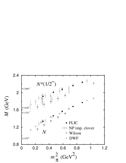
Figure 5: Masses of the nucleon ($N$) and the lowest $J^{P}={1\over 2}^{-}$ excitation (“$N^{*}$”). The FLIC and Wilson results are from the present analysis, with the DWF DWF and NP improved clover RICHARDS results shown for comparison. The empirical nucleon and low lying $N^{*}({1\over 2}^{-})$ masses are indicated by the asterisks along the ordinate.

Table 1: Values of $\kappa$ used in this analysis and the corresponding pion and nucleon resonance masses for the FLIC action with 4 sweeps of smearing at $\alpha=0.7$. Here $\kappa_{\rm cr}=0.1300$, and a string tension analysis gives $a=0.122(2)$ fm for $\sqrt{\sigma}=440$ MeV.

$\kappa$	$m_{\pi}a$	$m_{N_{1}}a$	$m_{N^{*}_{1}}a$	$m_{N^{*}_{2}}a$	$m_{N_{2}}a$
0.1260	0.5807(18)	1.0972(49)	1.388(14)	1.442(12)	1.676(12)
0.1266	0.5343(19)	1.0400(53)	1.340(16)	1.404(15)	1.642(13)
0.1273	0.4758(21)	0.9701(59)	1.286(19)	1.363(20)	1.605(15)
0.1279	0.4203(23)	0.9067(67)	1.244(25)	1.345(29)	1.580(18)
0.1286	0.3457(28)	0.8273(86)	1.186(33)	1.374(57)	1.571(26)

Figure 2 illustrates the effective mass plots of the correlation functions projected from the correlation matrix as in Eq. (56). The improved plateau behaviour is readily visible. Whereas in Fig. 1 the odd-parity effective masses are crossing at $t=6$ and have minimal mass splitting, significant mass splitting between the two states is already apparent at $t=6$ in Fig. 2. The covariance based $\chi^{2}/N_{\rm DF}$ indicates that acceptable plateaus in the effective mass plots start even earlier in some cases. The increase in mass splitting between the two negative parity states is more dramatic for $\Lambda^{*}_{c}$ than for the octet baryon interpolating fields. There the off diagonal elements of the correlation matrix are suppressed for the negative parity octet baryons, but not so for $\Lambda^{*}_{c}$. As a result, the projection of states has only only a small effect for the octet baryon interpolators and this is detailed in Section VIc.

Figs. 3 and 4 show the effective mass plots of the nucleon correlation functions $\chi_{1}\overline{\chi}_{1}$ and $\chi_{2}\overline{\chi}_{2}$ and following projection of the correlation matrix, respectively. Plots for the lightest quark mass considered are presented. The covariance matrix analysis of all quark masses indicates the following analysis windows in Euclidean time,

$$N_{1}\,,10-14 N_{1}^{*}\,,9-12\,;$$ ;

$$N_{2}^{*}\,,8-11 N_{2}\,,6-8\,.$$ ;

A comparison of Figs. 3 and 4 indicates that the correlation matrix analysis has a significantly smaller effect for the nucleon interpolators than the $\Lambda_{c}$ interpolators. This suggests that the states created by the interpolating fields $\chi_{1}$ and $\chi_{2}$ have good overlap with the two lowest-lying physical nucleon states.

VI.2 Resonance masses and lattice action dependence

In Fig. 5 we show the nucleon and $N^{*}({1\over 2}^{-})$ masses as a function of the pseudoscalar meson mass squared, $m_{\pi}^{2}$. The results of the new simulations are indicated by the filled squares for the FLIC action, and by the stars for the Wilson action (the Wilson points are obtained from a sample of 50 configurations). The values of $m_{\pi}^{2}$ correspond to $\kappa$ values given in Table 1.

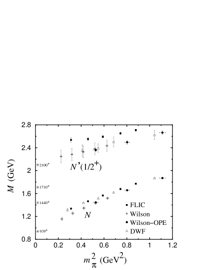
Figure 6: Masses of the nucleon, and the lowest $J^{P}={1\over 2}^{+}$ excitation (“$N^{\prime}$”). The FLIC results are compared with the earlier DWF DWF and Wilson-OPE LEIN1 analyses, as well as with the Wilson results from this analysis. The empirical nucleon and low lying $N^{*}({1\over 2}^{+})$ masses are indicated by asterisks.

Table 2: Interpolating field coefficients for the two positive parity $N^{1/2^{+}}$ states. The time slice $T$ at which the correlation matrix analysis is performed is indicated in the last column.

$\kappa$	$u_{1}^{a}$	$u_{2}^{a}$	$u_{1}^{b}$	$u_{2}^{b}$	$T$
0.1260	0.999(1)	0.001(1)	0.154(28)	0.846(28)	7
0.1266	0.997(2)	0.003(2)	0.112(59)	0.888(59)	8
0.1273	0.996(2)	0.004(2)	0.083(74)	0.917(74)	8
0.1279	0.993(3)	0.007(3)	0.049(99)	0.951(99)	8
0.1286	0.989(3)	0.011(3)	0.066(81)	0.934(81)	7

Table 3: Interpolating field coefficients for the two negative parity $N^{1/2^{-}}$ states. The eigenvalues of the correlation matrix analysis indicate that excited states spoil the eigenstate isolation for $\kappa$ values 0.1273 and 0.1279.

$\kappa$	$u_{1}^{a*}$	$u_{2}^{a*}$	$u_{1}^{b*}$	$u_{2}^{b*}$	$T$
0.1260	0.45(7)	0.55(7)	0.16(15)	–0.84(15)	8
0.1266	0.50(7)	0.50(7)	0.08(14)	–0.92(14)	8
0.1273	0.42(6)	0.58(6)	0.26(15)	–0.74(15)	7
0.1279	0.53(10)	0.47(10)	0.09(15)	–0.91(15)	7
0.1286	0.77(15)	0.23(15)	0.20(5)	0.80(5)	8

For comparison, we also show results from earlier simulations with domain wall fermions (DWF) DWF (open triangles), and a nonperturbatively (NP) improved clover action at $\beta=6.2$ RICHARDS . The scatter of the different NP improved results is due to different source smearing and volume effects: the open squares are obtained by using fuzzed sources and local sinks, the open circles use Jacobi smearing at both the source and sink, while the open diamonds, which extend to smaller quark masses, are obtained from a larger lattice ($32^{3}\times 64$) using Jacobi smearing. The empirical masses of the nucleon and the three lowest ${1\over 2}^{-}$ excitations are indicated by the asterisks along the ordinate.

There is excellent agreement between the different improved actions for the nucleon mass, in particular between the FLIC, DWF DWF and NP improved clover RICHARDS results. On the other hand, the Wilson results lie systematically low in comparison to these due to the large ${\cal O}(a)$ errors in this action FATJAMES . A similar pattern is repeated for the $N^{*}({1\over 2}^{-})$ masses. Namely, the FLIC, DWF and NP improved clover masses are in good agreement with each other, while the Wilson results again lie systematically lower. A mass splitting of around 400 MeV is clearly visible between the $N$ and $N^{*}$ for all actions, including the Wilson action, despite its poor chiral properties. Furthermore, the trend of the $N^{*}({1\over 2}^{-})$ data with decreasing $m_{\pi}$ is consistent with the mass of the lowest lying physical negative parity $N^{*}$ states.

Figure 6 shows the mass of the $J^{P}={1\over 2}^{+}$ states (the excited state is denoted by “$N^{\prime}(1/2^{+})$”). As is long known, the positive parity $\chi_{2}$ interpolating field does not have good overlap with the nucleon ground state LEIN1 and the correlation matrix results confirm this result, as discussed below. It has been speculated that $\chi_{2}$ may have overlap with the lowest ${1\over 2}^{+}$ excited state, the $N^{*}(1440)$ Roper resonance DWF . In addition to the FLIC and Wilson results from the present analysis, we also show in Fig. 6 the DWF results DWF , and results from an earlier analysis with Wilson fermions together with the operator product expansion LEIN1 . The physical values of the lowest three ${1\over 2}^{+}$ excitations of the nucleon are indicated by the asterisks.

The most striking feature of the data is the relatively large excitation energy of the $N^{\prime}({1\over 2}^{+})$, some 1 GeV above the nucleon. There is little evidence, therefore, that this state is the $N^{*}(1440)$ Roper resonance. While it is possible that the Roper resonance may have a strong nonlinear dependence on the quark mass at $m_{\pi}^{2}\lesssim 0.2$ GeV², arising from, for example, pion loop corrections, it is unlikely that this behaviour would be so dramatically different from that of the $N^{*}(1535)$ so as to reverse the level ordering obtained from the lattice. A more likely explanation is that the $\chi_{2}$ interpolating field does not have good overlap with either the nucleon or the $N^{*}(1440)$, but rather (a combination of) excited ${1\over 2}^{+}$ state(s).

Recall that in a constituent quark model in a harmonic oscillator basis, the mass of the lowest mass state with the Roper quantum numbers is higher than the lowest $P$-wave excitation. It seems that neither the lattice data (at large quark masses and with our interpolating fields) nor the constituent quark model have good overlap with the Roper resonance. Better overlap with the Roper is likely to require more exotic interpolating fields.

In Fig. 7 we show the ratio of the masses of the low-lying $N^{*}({1\over 2}^{-})$ and the nucleon. Once again, there is good agreement between the FLIC and DWF actions. However, the results for the Wilson action lie above the others, as do those for the anisotropic D₂₃₄ action LEE . The D₂₃₄ action has been mean-field improved, and uses an anisotropic lattice which is relatively coarse in the spatial direction ($a\approx 0.24$ fm). This is perhaps an indication of the need for nonperturbative or FLIC improvement.

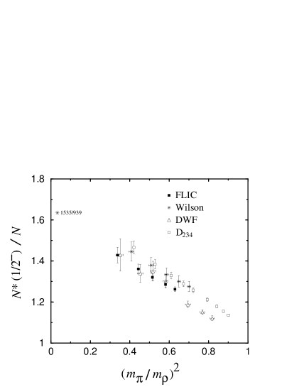
Figure 7: Ratio of the lowest $N^{*}({1\over 2}^{-})$ and nucleon masses. The FLIC and Wilson results are from the present analysis, with results from the D₂₃₄ LEE and DWF DWF actions shown for comparison. The empirical $N^{*}(1535)/N$ mass ratio is denoted by the asterisk.

VI.3 Resolving the resonances

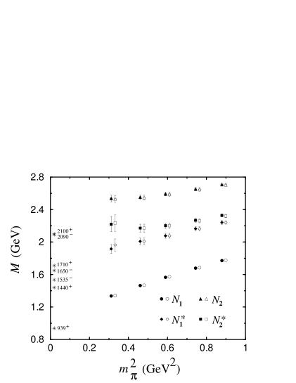
Figure 8: Masses of the $J^{P}={1\over 2}^{+}$ and ${1\over 2}^{-}$ nucleon states, for the FLIC action. The positive (negative) parity states are labeled $N_{1}$ ($N_{1}^{*}$) and $N_{2}$ ($N_{2}^{*}$). The results from the projection of the correlation matrix as discussed in Sec. VI.1 are shown by the filled symbols, whereas the results from the standard fits to the $\chi_{1}\overline{\chi}_{1}$ and $\chi_{2}\overline{\chi}_{2}$ correlation functions are shown by the open symbols (offset to the right for clarity). Empirical masses of the low lying ${1\over 2}^{\pm}$ states are indicated by the asterisks.

The mass splitting between the two lightest $N^{*}({1\over 2}^{-})$ states ($N^{*}(1535)$ and $N^{*}(1650)$) can be studied by considering the odd parity content of the $\chi_{1}$ and $\chi_{2}$ interpolating fields in Eqs. (6) and (7). Recall that the “diquarks” in $\chi_{1}$ and $\chi_{2}$ couple differently to spin, so that even though the correlation functions built up from the $\chi_{1}$ and $\chi_{2}$ fields will be made up of a mixture of many excited states, they will have dominant overlap with different states LEIN1 ; LL . By using the correlation-matrix techniques introduced in the previous section, we extract two separate mass states from the $\chi_{1}$ and $\chi_{2}$ interpolating fields. The results from the correlation matrix analysis are shown by the filled symbols in Fig. 8 and are compared to the standard “naive” fits performed directly on the diagonal correlation functions, $\chi_{1}\overline{\chi}_{1}$ and $\chi_{2}\overline{\chi}_{2}$, indicated by the open symbols.

Table 4: $\Sigma$ baryon resonance masses.

$\kappa$	$m_{\Sigma_{1}}a$	$m_{\Sigma^{*}_{1}}a$	$m_{\Sigma^{*}_{2}}a$	$m_{\Sigma_{2}}a$
0.1260	1.0765(50)	1.371(15)	1.432(13)	1.665(12)
0.1266	1.0400(53)	1.340(16)	1.404(15)	1.642(13)
0.1273	0.9966(57)	1.307(17)	1.371(17)	1.617(14)
0.1279	0.9589(62)	1.281(20)	1.349(21)	1.597(16)
0.1286	0.9149(72)	1.265(29)	1.332(28)	1.580(19)

Table 5: Interpolating field coefficients for the two $\Sigma^{1/2^{+}}$ states.

$\kappa$	$u_{1}^{a}$	$u_{2}^{a}$	$u_{1}^{b}$	$u_{2}^{b}$	$T$
0.1260	0.997(1)	0.003(1)	0.127(53)	0.873(53)	8
0.1266	0.997(2)	0.003(2)	0.112(59)	0.888(59)	8
0.1273	0.998(2)	0.002(2)	0.133(35)	0.867(35)	7
0.1279	0.997(2)	0.003(2)	0.121(41)	0.879(41)	7
0.1286	0.996(3)	0.004(3)	0.100(52)	0.900(52)	7

Table 6: Interpolating field coefficients for the two $\Sigma^{1/2^{-}}$ states. The eigenvalues of the correlation matrix analysis indicate that excited states spoil the eigenstate isolation for $\kappa$ values 0.1273 through 0.1286.

$\kappa$	$u_{1}^{a*}$	$u_{2}^{a*}$	$u_{1}^{b*}$	$u_{2}^{b*}$	$T$
0.1260	0.47(7)	0.53(7)	0.11(13)	–0.89(13)	8
0.1266	0.50(7)	0.50(7)	0.08(14)	–0.92(14)	8
0.1273	0.38(5)	0.62(5)	0.35(14)	–0.65(14)	7
0.1279	0.42(7)	0.58(7)	0.30(17)	–0.70(17)	7
0.1286	0.52(13)	0.48(13)	0.17(22)	–0.83(22)	7

The results indicate that indeed the $N^{*}({1\over 2}^{-})$ largely corresponding to the $\chi_{2}$ field (labeled “$N_{2}^{*}$”) lies above the $N^{*}({1\over 2}^{-})$ which can also be isolated via Euclidean time evolution with the $\chi_{1}$ field (“$N_{1}^{*}$”) alone. The masses of the corresponding positive parity states, associated with the $\chi_{1}$ and $\chi_{2}$ fields (labeled “$N_{1}$” and “$N_{2}$”, respectively) are shown for comparison. For reference, we also list the experimentally measured values of the low-lying ${1\over 2}^{\pm}$ states. It is interesting to note that the mass splitting between the positive parity $N_{1}$ and negative parity $N_{1,2}^{*}$ states (roughly 400–500 MeV) is similar to that between the $N_{1,2}^{*}$ and the positive parity $N_{2}$ state, reminiscent of a constituent quark–harmonic oscillator picture.

Table 7: $\Xi$ baryon resonance masses.

$\kappa$	$m_{\Xi_{1}}$ a	$m_{\Xi^{*}_{1}a}$	$m_{\Xi^{*}_{2}}a$	$m_{\Xi_{2}}a$
0.1260	1.0612(52)	1.358(15)	1.414(13)	1.653(12)
0.1266	1.0400(53)	1.340(16)	1.404(15)	1.642(13)
0.1273	1.0145(54)	1.320(16)	1.392(17)	1.630(14)
0.1279	0.9919(56)	1.302(18)	1.389(20)	1.622(15)
0.1286	0.9649(60)	1.281(20)	1.399(27)	1.618(24)

The interpolating coefficients for the two positive and negative parity states (see Eq. (47)), extracted via the procedure outlined in Section V.2, are given in Tables 3 and 3 for various $\kappa$ values. The coefficients corresponding to each mass state (labeled “$a$” or “$b$”) are normalised

Table 8: Interpolating field coefficients for the two $\Xi^{1/2^{+}}$ states.

$\kappa$	$u_{1}^{a}$	$u_{2}^{a}$	$u_{1}^{b}$	$u_{2}^{b}$	$T$
0.1260	0.999(1)	0.001(1)	0.146(30)	0.854(30)	7
0.1266	0.997(2)	0.003(2)	0.112(59)	0.888(59)	8
0.1273	0.996(2)	0.004(2)	0.105(64)	0.895(64)	8
0.1279	0.995(2)	0.005(2)	0.097(70)	0.903(70)	8
0.1286	0.993(2)	0.007(2)	0.076(83)	0.924(83)	8

Table 9: Interpolating field coefficients for the two $\Xi^{1/2^{-}}$ states. The eigenvalues of the correlation matrix analysis indicate that excited states spoil the eigenstate isolation for $\kappa$ values 0.1273 through 0.1286.

$\kappa$	$u_{1}^{a*}$	$u_{2}^{a*}$	$u_{1}^{b*}$	$u_{2}^{b*}$	$T$
0.1260	0.48(8)	0.52(8)	0.13(16)	–0.87(16)	8
0.1266	0.50(7)	0.50(7)	0.08(14)	–0.92(14)	8
0.1273	0.38(5)	0.62(5)	0.32(13)	–0.68(13)	7
0.1279	0.42(6)	0.58(6)	0.22(13)	–0.78(13)	7
0.1286	0.49(7)	0.51(7)	0.09(11)	–0.91(11)	7

so that the sum of their absolute values is 1,

$$|u_{1}^{a}|+|u_{2}^{a}| = 1\ ,$$ (58a)

$$|u_{1}^{b}|+|u_{2}^{b}| = 1\ ,$$ (58b)

and similarly for the coefficients $u_{1,2}^{a,b\ *}$ for the negative parity mass states. This normalisation allows one to readily identify the fraction of each interpolating field needed to construct a linear combination having maximum overlap with a particular baryon state. The last column in Tables 3 and 3 shows the time slice $T$ where the correlation matrix eigenvalue analysis is performed.

From Table 3 one immediately sees that the coefficient $u_{2}^{a}$, reflecting the fraction of $\chi_{2}$ required to isolate the ground state nucleon, is extremely small. This further supports the earlier observation that the $\chi_{2}$ interpolating field does not have good overlap with the nucleon ground state. Table 3 shows the coefficients for isolating the two lowest-energy negative-parity $N^{*}$ states using the $\chi_{1}$ and $\chi_{2}$ interpolating fields. A significant amount of mixing is observed between the two interpolating fields for the lower energy state, particularly at heavy quark masses. This result is anticipated by the long Euclidean time evolution required to achieve an acceptable $\chi^{2}/N_{\rm DF}$ for the $N_{1}^{*}$ effective mass illustrated in Fig. 3. The higher $N^{1/2^{-}}$ state, however, is dominated by the $\chi_{2}$ field, thus explaining the good effective mass plateau observed in Fig. 3 without the correlation matrix approach. Note that the most significant contribution to the $N_{2}^{*}$ state from $\chi_{1}$ is for the third quark mass when the correlation matrix analysis is performed at an early time slice and is spoiled by contamination from higher excited states. The most significant contribution at the preferred time slice, which also has the smallest errors, is for the lightest quark mass. It is for these reasons that we choose the lightest quark mass in Fig. 3 to illustrate the effective masses of the projected nucleon states.

Table 10: $\Lambda$ baryon resonance masses from the octet, $\Lambda^{8}$, interpolating field.

$\kappa$	$m_{\Lambda_{1}}a$	$m_{\Lambda^{*}_{1}}a$	$m_{\Lambda^{*}_{2}}a$	$m_{\Lambda_{2}}a$
0.1260	1.0801(50)	1.374(15)	1.427(13)	1.665(12)
0.1266	1.0400(53)	1.340(16)	1.404(15)	1.642(13)
0.1273	0.9910(56)	1.302(17)	1.380(19)	1.618(15)
0.1279	0.9464(61)	1.269(21)	1.373(26)	1.603(17)
0.1286	0.8904(72)	1.233(28)	1.410(47)	1.599(21)

Table 11: Interpolating field coefficients for the two positive parity $\Lambda^{8}$ states.

$\kappa$	$u_{1}^{a}$	$u_{2}^{a}$	$u_{1}^{b}$	$u_{2}^{b}$	$T$
0.1260	0.999(1)	0.001(1)	0.149(29)	0.851(29)	7
0.1266	0.997(2)	0.003(2)	0.112(59)	0.888(59)	8
0.1273	0.995(2)	0.005(2)	0.095(69)	0.905(69)	8
0.1279	0.993(2)	0.007(2)	0.070(85)	0.930(85)	8
0.1286	0.990(2)	0.010(2)	0.081(63)	0.919(63)	7

Table 12: Interpolating field coefficients for the two negative parity $\Lambda^{8}$ states. The eigenvalues of the correlation matrix analysis indicate that excited states spoil the eigenstate isolation for $\kappa$ values 0.1273 through 0.1286.

$\kappa$	$u_{1}^{a*}$	$u_{2}^{a*}$	$u_{1}^{b*}$	$u_{2}^{b*}$	$T$
0.1260	0.46(8)	0.54(8)	0.16(16)	–0.84(16)	8
0.1266	0.50(7)	0.50(7)	0.08(14)	–0.92(14)	8
0.1273	0.40(6)	0.60(6)	0.27(14)	–0.73(13)	7
0.1279	0.49(8)	0.51(8)	0.12(13)	–0.88(13)	7
0.1286	0.47(8)	0.53(8)	0.19(13)	–0.81(13)	6

Table 13: $\Lambda$ baryon resonance masses from the “common”, $\Lambda^{c}$, interpolating field.

$\kappa$	$m_{\Lambda_{1}}a$	$m_{\Lambda^{*}_{1}}a$	$m_{\Lambda^{*}_{2}}a$	$m_{\Lambda_{2}}a$
0.1260	1.0815(50)	1.334(13)	1.408(12)	1.662(11)
0.1266	1.0413(52)	1.301(14)	1.382(13)	1.638(12)
0.1273	0.9920(56)	1.262(16)	1.356(16)	1.611(12)
0.1279	0.9473(61)	1.226(18)	1.342(21)	1.590(13)
0.1286	0.8912(73)	1.181(21)	1.357(33)	1.570(15)

Table 14: Interpolating field coefficients for the two positive parity $\Lambda^{c}$ states.

$\kappa$	$u_{1}^{a}$	$u_{2}^{a}$	$u_{1}^{b}$	$u_{2}^{b}$	$T$
0.1260	1.000(2)	0.000(2)	0.282(51)	–0.718(51)	9
0.1266	0.997(2)	0.003(2)	0.291(55)	–0.709(55)	9
0.1273	0.994(2)	0.006(2)	0.278(26)	–0.722(26)	8
0.1279	0.990(2)	0.010(2)	0.279(18)	–0.721(18)	7
0.1286	0.983(3)	0.017(3)	0.278(13)	–0.722(13)	6

Table 15: Interpolating field coefficients for the two negative parity $\Lambda^{c}$ states. The correlation matrix analysis is successful for all $\kappa$ values.

$\kappa$	$u_{1}^{a*}$	$u_{2}^{a*}$	$u_{1}^{b*}$	$u_{2}^{b*}$	$T$
0.1260	0.54(2)	–0.46(2)	0.23(3)	0.77(3)	8
0.1266	0.53(2)	–0.47(2)	0.27(3)	0.73(3)	8
0.1273	0.52(1)	–0.48(1)	0.33(3)	0.67(3)	8
0.1279	0.51(1)	–0.49(1)	0.39(3)	0.61(3)	8
0.1286	0.49(1)	–0.51(1)	0.47(4)	0.53(4)	8

Turning to the strange sector, in Fig. 9 we show the masses of the positive and negative parity $\Sigma$ baryons calculated from the FLIC action compared with the physical masses of the known positive and negative parity states. The data for the masses of these states are listed in Table 4, and the interpolator coefficients for the two positive and negative parity states are given in Tables 6 and 6, respectively. The pattern of mass splittings is similar to that found in Fig. 8 for the nucleon. Namely, the ${1\over 2}^{+}$ state associated with the $\chi_{1}$ field appears consistent with the empirical $\Sigma(1193)$ ground state, while the ${1\over 2}^{+}$ state associated with the $\chi_{2}$ field lies significantly above the observed first (Roper-like) ${1\over 2}^{+}$ excitation, $\Sigma^{*}(1660)$. There is also evidence for a mass splitting between the two negative parity states, similar to that in the nonstrange sector. The behaviour of the interpolator coefficients for the $\Sigma^{1/2^{+}}$ and $\Sigma^{1/2^{-}}$ states is also similar to that for the nucleon in Tables 3 and 3. Namely, while the positive parity ground state is dominated by the $\chi_{1}$ interpolating field, there is considerable mixing between the $\chi_{1}$ and $\chi_{2}$ fields for the lowest negative parity state, with the higher $\Sigma^{1/2^{-}}$ state receiving a dominant contribution from $\chi_{2}$.

The spectrum of the strangeness –2 positive and negative parity $\Xi$ hyperons is displayed in Fig. 10, with data given in Table 7, and the interpolator coefficients for the $\Xi^{1/2^{+}}$ and $\Xi^{1/2^{-}}$ states in Tables 9 and 9, respectively. Once again, the pattern of calculated masses repeats that found for the $\Sigma$ and $N$ masses in Figs. 8 and 9, and for the respective coupling coefficients. The empirical masses of the physical $\Xi^{*}$ baryons are denoted by asterisks. However, for all but the ground state $\Xi(1318)$, the $J^{P}$ values are not known.

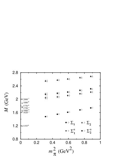
Figure 9: As in Fig. 8 but for the $\Sigma$ baryons.

Figure 10: As in Fig. 8 but for the $\Xi$ baryons. The $J^{P}$ values of the excited states marked with “?” are undetermined.

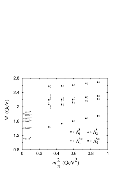
Figure 11: As in Fig. 8 but for the $\Lambda$ states obtained using the $\Lambda^{8}$ interpolating field.

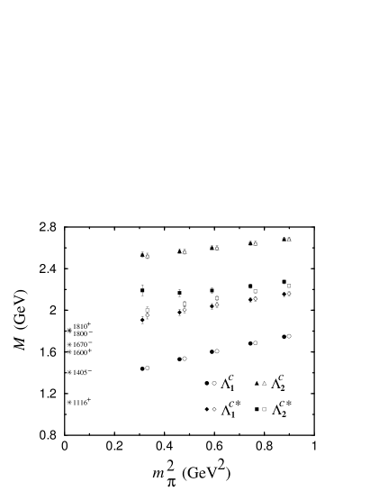
Figure 12: As in Fig. 8 but for the $\Lambda$ states obtained using the $\Lambda^{c}$ interpolating field.

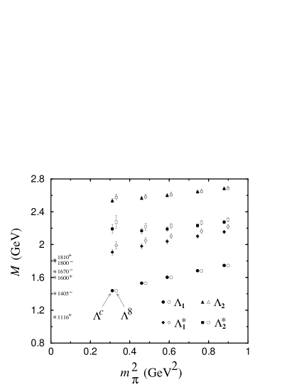
Figure 13: Masses of the positive and negative parity $\Lambda$ states, for the octet $\Lambda^{8}$ (open symbols) and “common” $\Lambda^{c}$ (filled symbols) interpolating fields with the FLIC action. The positive (negative) parity states labeled $\Lambda_{1}$ ($\Lambda_{1}^{*}$) and $\Lambda_{2}$ ($\Lambda_{2}^{*}$) are the two states obtained from the correlation matrix analysis of the $\chi_{1}^{\Lambda}$ and $\chi_{2}^{\Lambda}$ interpolating fields. Empirical masses of the low lying ${1\over 2}^{\pm}$ states are indicated by the asterisks.

Finally, we consider the $\Lambda$ hyperons. In Figs. 11 and 12 we compare results obtained from the $\Lambda^{8}$ and $\Lambda^{c}$ interpolating fields, respectively, using the two different techniques for extracting masses. The data are given in Tables 10 and 13, respectively. A direct comparison between the positive and negative parity masses for the $\Lambda^{8}$ (open symbols) and $\Lambda^{c}$ (filled symbols) states extracted from the correlation matrix analysis, is shown in Fig. 13. A similar pattern of mass splittings to that for the $N^{*}$ spectrum of Fig. 8 is observed. In particular, the negative parity $\Lambda_{1}^{*}$ state (diamonds) lies $\sim 400$ MeV above the positive parity $\Lambda_{1}$ ground state (circles), for both the $\Lambda^{8}$ and $\Lambda^{c}$ fields. There is also clear evidence of a mass splitting between the $\Lambda_{1}^{*}$ (diamonds) and $\Lambda_{2}^{*}$ (squares).

Using the naive fitting scheme (open symbols in Figs. 11 and 12), misses the mass splitting between $\Lambda_{1}^{*}$ and $\Lambda_{2}^{*}$ for the “common” interpolating field. Only after performing the correlation matrix analysis is it possible to resolve two separate mass states, as seen by the filled symbols in Fig. 12. This may be an indication that the physics responsible for the mass splitting between the negative parity $\Lambda^{*}(1670)$ and $\Lambda^{*}(1800)$ states is suppressed in the $\Lambda^{c}$ interpolating field. This is also evidenced by comparing the interpolator coefficients for the positive and negative parity $\Lambda^{8}$ and $\Lambda^{c}$ states, in Tables 12 and 12, and 15 and 15, respectively. While the couplings for the $\Lambda^{8}$ for both the positive parity states are similar to those for the nucleon and other hyperons, there is more prominent mixing for the case of the $\Lambda^{c}$. In particular, there is notably stronger mixing for the higher mass negative parity state in the case of the $\Lambda^{c}$ compared with the corresponding $\Lambda^{8}$ state. The $\chi_{2}^{\Lambda^{8}}$ contributes $\sim 80$–90% of the strength compared to $\sim 50$–60% for the $\chi_{2}^{\Lambda^{c}}$. The interpolator coefficients are precisely determined in the $\Lambda^{c}$ correlation matrix analysis. As for the other baryons, there is little evidence that the $\Lambda_{2}$ (triangles) has any significant overlap with the first positive parity excited state, $\Lambda^{*}(1600)$ (c.f. the Roper resonance, $N^{*}(1440)$, in Fig. 8).

While it seems plausible that nonanalyticities in a chiral extrapolation MASSEXTR of $N_{1}$ and $N_{1}^{*}$ results could eventually lead to agreement with experiment, the situation for the $\Lambda^{*}(1405)$ is not as compelling. Whereas a 150 MeV pion-induced self energy is required for the $N_{1},\ N_{1}^{*}$ and $\Lambda_{1}$, 400 MeV is required to approach the empirical mass of the $\Lambda^{*}(1405)$. This may not be surprising for the octet fields, as the $\Lambda^{*}(1405)$, being an SU(3) flavour singlet, may not couple strongly to an SU(3) octet interpolating field. Indeed, there is some evidence of this in Fig. 13. This large discrepancy of 400 MeV suggests that relevant physics giving rise to a light $\Lambda^{*}(1405)$ may be absent from simulations in the quenched approximation. The behaviour of the $\Lambda_{1,2}^{*}$ states may be modified at small values of the quark mass through nonlinear effects associated with Goldstone boson loops including the strong coupling of the $\Lambda^{*}(1405)$ to $\Sigma\pi$ and $\bar{K}N$ channels. While some of this coupling will survive in the quenched approximation, generally the couplings are modified and suppressed YOUNG ; SHARPE . It is also interesting to note that the $\Lambda_{1}^{*}$ and $\Lambda_{2}^{*}$ masses display a similar behaviour to that seen for the $\Xi_{1}^{*}$ and $\Xi_{2}^{*}$ states, which are dominated by the heavier strange quark. Alternatively, the study of more exotic interpolating fields may indicate the the $\Lambda^{*}(1405)$ does not couple strongly to $\chi_{1}$ or $\chi_{2}$. Investigations at lighter quark masses involving quenched chiral perturbation theory will assist in resolving these issues.

VII Conclusion

We have presented the first results for the excited baryon spectrum from lattice QCD using an ${\cal O}(a^{2})$ improved Luscher-Weise gauge action Luscher:1984xn and an ${\cal O}(a)$-improved Fat-Link Irrelevant Clover (FLIC) quark action in which only the links of the irrelevant dimension five operators are smeared FATJAMES . The FLIC action provides a new form of nonperturbative ${\cal O}(a)$ improvement in which ${\cal O}(a)$ errors are eliminated and ${\cal O}(a^{2})$ errors are very small QNPproc . The simulations have been performed on a $16^{3}~{}\times~{}32$ lattice at $\beta=4.60$, providing a lattice spacing of $a=0.122(2)$ fm. The analysis is based on a set of 400 configurations generated on the Orion supercomputer at the University of Adelaide.

Good agreement is obtained between the FLIC and other improved actions, including the nonperturbatively improved clover RICHARDS and domain wall fermion (DWF) DWF actions, for the nucleon and its chiral partner, with a mass splitting of $\sim 400$ MeV. Our results for the $N^{*}({1\over 2}^{-})$ improve on those using the D₂₃₄ LEE and Wilson actions. Despite strong chiral symmetry breaking, the results with the Wilson action are still able to resolve the splitting between the chiral partners of the nucleon. Using the two standard nucleon interpolating fields, we also confirm earlier observations LL of a mass splitting between the two nearby ${1\over 2}^{-}$ states. We find no evidence of overlap with the ${1\over 2}^{+}$ Roper resonance.

In the strange sector, we have investigated the overlap of various $\Lambda$ interpolating fields with the low-lying ${1\over 2}^{\pm}$ states. Once again a clear mass splitting of $\sim 400$ MeV between the octet $\Lambda$ and its parity partner is seen, with evidence of a mass splitting between the two low-lying odd-parity states We find no evidence of strong overlap with the ${1\over 2}^{+}$ “Roper” excitation, $\Lambda^{*}(1600)$. The empirical mass suppression of the $\Lambda^{*}(1405)$ is not evident in these quenched QCD simulations, possibly suggesting an important role for the meson cloud of the $\Lambda^{*}(1405)$ and/or a need for more exotic interpolating fields.

We have not attempted to extrapolate the lattice results to the physical region of light quarks, since the nonanalytic behaviour of $N^{*}$’s near the chiral limit is not as well studied as that of the nucleon MASSEXTR ; YOUNG ; Young:2002ib . It is vital that future lattice $N^{*}$ simulations push closer towards the chiral limit. On a promising note, our simulations with the 4 sweep FLIC action are able to reach relatively low quark masses ($m_{q}\sim 60$–70 MeV) already. Our discussion of quenching effects is limited to a qualitative level until the formulation of quenched chiral perturbation theory for ${1\over 2}^{-}$ baryon resonances is established CROUCH or dynamical fermion simulations are completed. Experience suggests that dynamical fermion results will be shifted down in mass relative to quenched results, with increased downward curvature near the chiral limit YOUNG . It will be fascinating to confront this physics with both numerical simulation and chiral nonanalytic approaches.

In order to further explore the origin of the Roper resonances or the $\Lambda^{*}(1405)$, more exotic interpolating fields involving higher Fock states, or nonlocal operators should be investigated. Finally, the present $N^{*}$ mass analysis will be extended in future to include $N\to N^{*}$ transition form factors through the calculation of three-point correlation functions.

- (1) S. Capstick and W. Roberts, Prog. Part. Nucl. Phys. 45 (2000) S241, nucl-th/0008028.
- (2) N. Isgur and G. Karl, Phys. Lett. B 72 (1977) 109; Phys. Rev. D 19 (1979) 2653; N. Isgur, ibid 62 (2000) 054026; nucl-th/0007008.
- (3) P. A. M. Guichon, Phys. Lett. B 164 (1985) 361.
- (4) O. Krehl, C. Hanhart, S. Krewald and J. Speth, Phys. Rev. C 62 (2000) 025207, nucl-th/9911080.
- (5) Z.-P. Li, V. Burkert and Z.-J. Li, Phys. Rev. D 46 (1992) 70; C. E. Carlson and N. C. Mukhopadhyay, Phys. Rev. Lett. 67 (1991) 3745.
- (6) R. H. Dalitz and J. G. McGinley, in Low and Intermediate Energy Kaon-Nucleon Physics, ed. E. Ferarri and G. Violini (Reidel, Boston, 1980), p.381; R. H. Dalitz, T.C. Wong and G. Rajasekaran, Phys. Rev. 153 (1967) 1617; E. A. Veit, B. K. Jennings, R. C. Barrett and A. W. Thomas, Phys. Lett. B 137 (1984) 415; E. A. Veit, B. K. Jennings, A. W. Thomas and R. C. Barrett, Phys. Rev. D 31 (1985) 1033; P. B. Siegel and W. Weise, Phys. Rev. C 38 (1988) 2221; N. Kaiser, P. B. Siegel and W. Weise, Nucl. Phys. A594 (1995) 325; E. Oset, A. Ramos and C. Bennhold, Phys. Lett. B 527 (2002) 99 [Erratum-ibid. B 530 (2002) 260] nucl-th/0109006.
- (7) D. B. Leinweber, A. W. Thomas, K. Tsushima and S. V. Wright, Phys. Rev. D 61 (2000) 074502, hep-lat/9906027.
- (8) R. D. Young, D. B. Leinweber, A. W. Thomas and S. V. Wright, Phys. Rev. D 66 (2002) 094507, hep-lat/0205017.
- (9) L. Y. Glozman and D. O. Riska, Phys. Rep. 268 (1996) 263; L. Y. Glozman, Phys. Lett. B 494 (2000) 58.
- (10) N. Isgur, Phys. Rev. D 62 (2000) 054026, nucl-th/9908028.
- (11) A. W. Thomas and G. Krein, Phys. Lett. B 456 (1999) 5; ibid. B 481 (2000) 21.
- (12) S. Capstick and N. Isgur, Phys. Rev. D 34 (1986) 2809.
- (13) C. L. Schat, J. L. Goity and N. N. Scoccola, Phys. Rev. Lett. 88 (2002) 102002, hep-ph/0111082; C. E. Carlson, C. D. Carone, J. L. Goity and R. F. Lebed, Phys. Rev. D 59 (1999) 114008; J. L. Goity, Phys. Lett. B 414 (1997) 140; D. Pirjol and C. Schat, hep-ph/0301187.
- (14) D. B. Leinweber, Ann. Phys. 198 (1990) 203.
- (15) D. B. Leinweber, Phys. Rev. D 47 (1993) 5096, hep-ph/9302266.
- (16) J. M. Zanotti et al. [CSSM Lattice Collaboration], Phys. Rev. D 65 (2002) 074507, hep-lat/0110216; Nucl. Phys. Proc. Suppl. 109 (2002) 101, hep-lat/0201004.
- (17) T. DeGrand [MILC collaboration], Phys. Rev. D 60 (1999) 094501, hep-lat/9903006.
- (18) D. B. Leinweber, Phys. Rev. D 51 (1995) 6383, nucl-th/9406001.
- (19) M. W. Hecht and T. A. DeGrand, Phys. Lett. B 275 (1992) 435; T. A. DeGrand and M. W. Hecht, Phys. Rev. D 46 (1992) 3937, hep-lat/9206011.
- (20) F. X. Lee and D. B. Leinweber, Nucl. Phys. Proc. Suppl. 73 (1999) 258.
- (21) F. X. Lee, Nucl. Phys. Proc. Suppl. 94 (2001) 251.
- (22) S. Sasaki, T. Blum and S. Ohta, Phys. Rev. D 65 (2002) 074503, hep-lat/0102010.
- (23) D. G. Richards, Nucl. Phys. Proc. Suppl. 94 (2001) 269; M. Göckeler et al. [QCDSF Collaboration], Phys. Lett. B 532 (2002) 63, hep-lat/0106022; D.G. Richards et al., [LHPCollaboration], Nucl. Phys. Proc. Suppl. 109 (2002) 89, hep-lat/0112031.
- (24) N. Nakajima, H. Matsufuru, Y. Nemoto and H. Suganuma, hep-lat/0204014.
- (25) F. X. Lee et al., hep-lat/0208070.
- (26) C. Allton et al., in preparation.
- (27) D. B. Leinweber, R. W. Woloshyn and T. Draper, Phys. Rev. D 43 (1991) 1659.
- (28) K. Bowler et al., Nucl. Phys. B240 (1984) 213.
- (29) K. Symanzik, Nucl. Phys. B226 (1983) 187.
- (30) F. D. Bonnet, D. B. Leinweber and A. G. Williams, J. Comput. Phys. 170 (2001) 1, hep-lat/0001017.
- (31) R. G. Edwards, U. M. Heller and T. R. Klassen, Nucl. Phys. B 517 (1998) 377, hep-lat/9711003.
- (32) M. Falcioni, M. Paciello, G. Parisi and B. Taglienti, Nucl. Phys. B251 (1985) 624; M. Albanese et al., Phys. Lett. B 192 (1987) 163.
- (33) B. Sheikholeslami and R. Wohlert, Nucl. Phys. B259, 572 (1985).
- (34) J. J. Sakurai, “Advanced Quantum Mechanics” (Addison-Wesley, 1982).
- (35) S. Bilson-Thompson, F. D. Bonnet, D. B. Leinweber and A. G. Williams, Nucl. Phys. Proc. Suppl. 109 (2002) 116, hep-lat/0112034; S. O. Bilson-Thompson, D. B. Leinweber and A. G. Williams, to appear in Annals of Physics, hep-lat/0203008.
- (36) S. Gusken, Nucl. Phys. Proc. Suppl. 17 (1990) 361.
- (37) C. McNeile and C. Michael, Phys. Rev. D 63 (2000) 114503, hep-lat/0010019.
- (38) J. N. Labrenz and S. R. Sharpe, Phys. Rev. D 54 (1996) 4595, hep-lat/9605034.
- (39) M. Luscher and P. Weisz, Commun. Math. Phys. 97, 59 (1985) [Erratum-ibid. 98, 433 (1985)].
- (40) D. B. Leinweber et al., nucl-th/0211014; J. M. Zanotti et al., in preparation.
- (41) R. D. Young, D. B. Leinweber and A. W. Thomas, arXiv:hep-lat/0212031.
- (42) B. Crouch, D. B. Leinweber, D. Morel and A. W. Thomas, in preparation.