Abstract

We propose to consider lattice monopoles in gluodynamics as continuum monopoles blocked to the lattice. In this approach the lattice is associated with a measuring device consisting of finite–sized detectors of monopoles (lattice cells). Thus a continuum monopole theory defines the dynamics of the lattice monopoles. We apply this idea to the static monopoles in high temperature gluodynamics. We show that our suggestion allows to describe the numerical data both for the density of the lattice monopoles and for the lattice monopole action in terms of a continuum Coulomb gas model.

* Presented by the first author at the NATO Advanced Research Workshop

”Confinement, Topology, and other Non-Perturbative Aspects of QCD”,

Stará Lesná, High Tatra Mountains (Slovakia), January 21-27, 2002

ITEP-LAT/2002-01

KANAZAWA-02-03

17 February, 2002

1 Introduction

One of the most successful approaches to the confinement phenomena in QCD is the based on the so–called dual superconductor mechanism [1]. The key role in the mechanism is played by Abelian monopoles which are identified with the help of the Abelian projection method [2] based on the partial gauge fixing of non–Abelian gauge symmetry up to a residual Cartan (Abelian) subgroup. The monopoles appear in the theory due to compactness of the Cartan subgroup. According to the numerical results [3] the monopoles are condensed in the low temperature (confinement) phase. The condensation of the monopoles leads to formation of the chromoelectric string which implies confinement of color. The importance of the Abelian monopoles is stressed by the Abelian dominance phenomena which was first observed in the lattice $SU(2)$ gluodynamics. In the so-called Maximal Abelian projection the monopoles make a dominant contribution to the zero temperature string tension [4]. At high temperatures, (deconfinement phase) the monopoles are responsible for the spatial string tension [5].

We propose to describe the dynamics of the Abelian monopoles in the $SU(2)$ gluodynamics considering the lattice as a kind of a ”monopole detector”. For the sake of simplicity we are working in the deconfinement phase dominated by static monopoles while monopoles running in spatial directions are suppressed. We investigate the physics of the static monopole currents which is effectively three dimensional.

2 Ideology

We suppose that the lattice with a finite lattice spacing $b$ is embedded in the continuum space-time. Each lattice cell, $C_{s}$, detects the total magnetic charge, $k_{s}$, of ”continuum” monopoles inside it:

$$k_{s}=\int\limits_{C_{s}}\mbox{d}^{3}x\,\rho(x)\,,\qquad\rho(x)=\sum_{a}q_{a}\,\delta^{(a)}(x-x^{(a)})\,,$$ (1)

where $\rho$ is the density of the continuum monopoles, $q_{a}$ and $x_{a}$ is the position and the charge (in units of a fundamental magnetic charge, $g_{M}$) of $a^{\mathrm{th}}$ continuum monopole. We stress the difference between continuum and lattice monopoles: the continuum monopoles are fundamental objects while the lattice monopoles are associated with non–zero magnetic charges of continuum monopoles located inside lattice cells, $k_{s}\neq 0$.

Before going into details we mention that our approach is similar to the blocking of the monopole degrees of freedom from fine to coarser lattices [6], which allows to define perfect quantum actions for topological defects. Another similarity can be observed with ideas of Ref. [7] where the blocking of the continuum fields to the lattice was proposed. Our approach is based on blocking of the continuum topological defects to the lattice, and, as a result, is more suitable for the investigation of the lattice monopoles. Indeed, blocking of the fields [7] leads to non–integer lattice magnetic currents which makes a comparison of the numerical results with the analytical predictions difficult.

Below we show that properties of the Abelian lattice monopoles – found in numerical simulations of hot $SU(2)$ gluodynamics – can be described by the continuum blocking proposed above. Suppose the dynamics of the continuum monopoles in the high temperature gluodynamics is governed by the standard $3D$ Coulomb gas model:

$${\cal Z}=\sum\limits_{N=0}^{\infty}\frac{\zeta^{N}}{N!}\Biggl{[}\prod\limits^{N}_{a=1}\int\mbox{d}^{3}x^{(a)}\sum\limits_{q_{a}=\pm 1}\Biggr{]}\exp\Bigl{\{}-\frac{g^{2}_{M}}{2}\sum\limits_{\stackrel{{\scriptstyle a,b=1}}{{a\neq b}}}^{N}q_{a}q_{b}\,D(x^{(a)}-x^{(b)})\Bigr{\}}\,,$$ (2)

where $\zeta$ is the so–called fugacity parameter and $D(x)$ is the inverse Laplacian in continuum. In this simple model the continuum monopoles are supposed to be point–like while the monopole core in $SU(2)$ gluodynamics is of a finite size [8]. However our results presented below show that this simplification works at high temperatures.

Below we choose the v.e.v. of the continuum monopole density, $\rho$, and the Debye mass, $m_{D}$, as suitable parameters of the continuum model (instead of $g_{M}$ and $\zeta$). In the leading order of the dilute gas approximation we have [9]: $\rho=2\zeta$ and $m_{D}=g_{M}\sqrt{2\zeta}$. It is worth mentioning that the $3D$ Debye mass corresponds to a magnetic screening mass in four dimensions.

We are interested in basic quantities characterizing the lattice monopoles: the v.e.v. of the squared magnetic charge, $\langle k^{2}_{s}\rangle$, and the monopole action, $S_{mon}(k)$. In addition to the parameters of the continuum model both these quantities should depend on the lattice monopole size, $b$. Note that we study the quantity $\langle k^{2}_{s}\rangle$ instead of the density, $\langle|k_{s}|\rangle$, since the analytical treatment of the density is difficult. However philosophically both these quantities are equivalent.

In the dilute gas approximation we get [10]:

$$\langle k^{2}_{s}\rangle(b)=\rho\,b^{3}\cdot P(b/\lambda_{D},L)\,,$$

$$P(\mu,L)=\frac{1}{L^{3}}\,\sum\limits_{\vec{q}\in{Z\!\!\!Z}}\frac{{\vec{u}}^{2}}{{\vec{u}}^{2}+\mu^{2}}\,\prod^{3}_{i=1}{\Biggl{[}\frac{2\sin[u_{i}(q)/2]}{u_{i}(q)}\Biggr{]}}^{2}\,,\quad u_{i}(q)=\frac{2\pi q_{i}}{L}\,,$$

where $L$ is the lattice size. The scale for the monopole size is given by the (magnetic) Debye screening length, $\lambda_{D}=1/m_{D}$. In a leading order we get for small and large lattice cubes:

$$\langle k^{2}_{s}\rangle(b)=\left\{\begin{array}[]{ll}\rho\cdot b^{3}+\cdots\,,&b\ll\lambda_{D}\,;\\ C\cdot\rho\,\lambda_{D}\cdot b^{2}+\cdots\,,&b\gg\lambda_{D}\,.\end{array}\right.$$ (5)

This expression is written in a thermodynamic limit where $C\approx 2.94$.

Analogously we may derive an effective action for the monopoles. Substituting the unity,

$$1=\prod\limits_{s}\sum\limits_{k_{s}\in{Z\!\!\!Z}}\delta\Biggl{(}k_{s}-\int_{C_{s}}\mbox{d}^{3}x\,\rho(x)\Biggr{)}\,,$$ (6)

into the Coulomb gas partition function (2) and integrating over all continuum monopoles we get in the dilute gas approximation [10]:

$$Z = \sum_{k\in{Z\!\!\!Z}}e^{-S_{mon}(k)}\,,\,\,\,S_{mon}(k)=\frac{1}{2\rho\,b^{3}}\sum\limits_{s,s^{\prime}}k_{s}\,{\cal F}_{s,s^{\prime}}(b/\lambda_{D})\,k_{s^{\prime}}\,,$$

$${\cal F}_{s,s^{\prime}}(\mu) = \frac{1}{L^{3}}\sum\limits^{L}_{\vec{m}=0}\,{\cal F}^{-1}\left(\frac{2\pi\vec{m}}{L},\mu\right)\cdot\exp\Bigl{\{}2\pi i(\vec{s}-\vec{s}\,^{\prime},\vec{m})/L\Bigr{\}}\,,$$

$${\cal F}(\vec{u},\mu) = \sum_{\vec{r}\in{Z\!\!\!Z}}\sum_{i=1}^{3}\frac{4\,\sin^{2}(u_{i}/2)}{(\vec{u}+2\pi\vec{r})^{2}+\mu^{2}}\,\prod^{3}_{\stackrel{{\scriptstyle j=1}}{{j\neq i}}}{\left(\frac{2\sin(u_{j}/2)}{u_{j}+2\pi r_{j}}\right)}^{2}\,,$$

where we omit higher–order corrections. According to this equation the leading order contribution to the monopole action is quadratic in monopole fields.

Similarly to the density of the squared monopole charge the monopole action depends on the ratio $b/\lambda_{D}$:

$$S_{mon}(k)=\left\{\begin{array}[]{lll}\frac{1}{4\rho}\cdot\frac{1}{b^{3}}\cdot\sum\limits_{s}k^{2}_{s}+\cdots\,,&b\ll\lambda_{D}\,;\\ \frac{1}{4\rho\,\lambda_{D}}\cdot\frac{1}{b^{2}}\cdot\sum\limits_{s,s^{\prime}}k_{s}\,D_{s,s^{\prime}}\,k_{s^{\prime}}+\cdots\,,&b\gg\lambda_{D}\,,\end{array}\right.$$ (9)

where $D_{s,s^{\prime}}$ is the inverse Laplacian on the lattice. Leading contribution to the monopole action is given by the massive (Coulomb) terms for small (large) lattice monopoles.

3 Analytics vs. Numerics

To study numerically the monopoles of various lattice sizes we use the extended monopole construction [11]. The size of the extended monopole is $b=na$, where $n$ is the lattice blocking size and $a$ is the lattice spacing of the fine lattice on which the fields of the $SU(3)$ gluodynamics are defined. We study only the static components, $k_{4}$, of the $4D$ monopole currents, $k_{\mu}$. The lattice blocking is performed only in spatial directions, $n_{s}=1\dots 8$. We simulate $SU(2)$ gluodynamics on the lattices $48^{3}\times L_{t}$ with $L_{t}=4\dots 12$ at temperatures $T/T_{c}=1.6\dots 4.8$. The size of the lattice monopoles is measured in terms of the zero temperature string tension, $\sigma_{T=0}$.

First we check the density of squared lattice monopole charge $vs.$ lattice monopole size, $b$, Figure 1.

(a) (b)

Figure 1.  : The ratio of the squared magnetic charge density and $b^{2}$, $\langle k^{2}(b)\rangle/b^{2}$, $vs.$ lattice monopole size, $b$, at (a) $T=1.6\,T_{c}$ and (b) $T=4.8\,T_{c}$.

According to eq.(5) the function $\langle k^{2}(b)\rangle/b^{2}$ must vanish at small monopole sizes and tend to constant at large $b$. This behaviour can be observed in our numerical data, Figure 1, up to some jumps for densities with different $n_{s}$. We ascribe these jumps to the lattice artifacts emerged due to finiteness of the fine lattice spacing, $a$, and finite volume effects. In Figure 1 the monopole size, $b$, is measured in units of the zero string tension, $\sigma_{T=0}$. The large-$b$ asymptotics of $\langle k^{2}(b)\rangle/b^{2}$ is approximated by averaging of the appropriate $n_{s}=8$ data. According to eq.(5) the large-$b$ asymptotics can be used to extract the dimensionless quantity,

$$R(T)=\frac{\sigma_{T=0}}{\lambda_{D}(T)\,\rho(T)}\,,$$ (10)

which is discussed in the next Section.

The monopole action for the static monopole currents, $k_{s}\equiv k_{s,4}$, at high temperatures was found numerically in Ref. [12]. The leading order terms in the action are quadratic:

$$S_{mon}(k)=\sum_{i}f_{i}\,S_{i}(k)\,,$$ (11)

where $S_{i}$ are two–point operators of the monopole charges (see Ref. [12] for details). An example of the monopole action for certain parameters is shown in Figure 2(a). In the same Figure we show the fitting of the action by the Coulomb action,

$$S_{mon}(k)=C_{C}\cdot\sum\limits_{s,s^{\prime}}k_{s}\,D_{s,s^{\prime}}\,k_{s^{\prime}}\,,$$ (12)

which follows from eq.(9). Here $C_{C}$ is the fitting parameter. This one-parametric fit works almost perfectly.

According to eq.(9) the pre-Coulomb coefficient $C_{C}(b,T)$ at sufficiently large monopole size , $b\gg\lambda_{D}$, must scale as follows:

$$C_{C}(b,T)=R(T)\cdot b^{-2}\,,$$ (13)

where $R$ is defined in eq.(10). We present the data for the pre-Coulomb coefficient and the corresponding one-parameter fits (13) in Figure 2(b). The agreement between the data and the fits is very good.

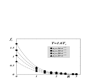
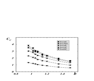
(a) (b)

Figure 2.  : (a) Two–point coupling constants, $f_{i}$, of the monopole action $vs.$ the distance between the lattice points, $r$ (in lattice units). The numerical data corresponds to $T=1.6T_{c}$, $n_{s}=6$ and various spatial spacings, $a_{s}$, of the fine lattice. The fits by the Coulomb interaction (12) are visualized by the dashed lines. (b) The pre-Coulomb coupling $C_{C}$ and the fits of $C_{C}$ by eq. (13) are shown for various temperatures, $T$.

4 Check of Coulomb gas picture

In this Section we present our results for the quantity $R$, eq.(10), which we have obtained both from the large–$b$ behaviour of the density $\langle k^{2}(b)\rangle$ and from the monopole action (in these cases we call the quantity $R$ as $R_{\rho}$ and $R_{act}$, respectively). From a numerical point of view the quantities $R_{\rho}$ and $R_{act}$ are independent. Thus a natural condition of a self–consistency of our approach is $R_{\rho}=R_{act}$. We check the self–consistency in Figure 3(a) plotting the ratio of these quantities. It is clearly seen that the ratio is independent on the temperature and very close to unity, as expected. The details of our calculations and further discussions will be presented in Ref. [10].

(a) (b)

Figure 3.  : (a) Check of self–consistency: the ratio of the quantities $R$, eq.(10) obtained from the lattice monopole action and the monopole density; (b) Check of the dilute Coulomb gas picture: quantity $R_{sp}$, eq.(14), obtained from the lattice monopole density.

Another interesting quantity is the ratio

$$R_{sp}(T)=\frac{\sigma_{sp}(T)}{\lambda_{D}(T)\,\rho(T)}\equiv R(T)\cdot\frac{\sigma_{sp}(T)}{\sigma_{T=0}}\,,$$ (14)

where $\sigma_{sp}$ is the spatial string tension. In the dilute Coulomb gas of monopoles we have the following relations [9]:

$$m_{D}\equiv\lambda^{-1}_{D}=g_{M}\,\sqrt{\rho}\,,\quad\sigma=\frac{8}{g_{M}}\sqrt{\rho}\,,$$ (15)

which imply $R_{sp}=8$. Using results of Ref. [13] for the spatial string tension in hot gluodynamics, $\sigma_{sp}(T)$, we get the quantity $R_{sp}$ as a function of the temperature, $T$, Figure 3(b). If the Coulomb picture works then $R_{sp}$ should be close to $8$. From Figure 3(b) we conclude that this is indeed the case at sufficiently large temperatures.

5 Conclusion

In order to describe the lattice monopole dynamics we have proposed to consider the lattice as a measuring device for the continuum monopoles. We have suggested that at high temperatures the static lattice monopoles can be described by a continuum Coulomb gas model. As a result we are able to draw the following conclusions:

• The continuum Coulomb gas model can describe the results of the Monte Carlo simulations for the density and action of the lattice monopoles. The dependence of these quantities on the physical sizes of the lattice monopoles is in agreement with the analytical predictions.

• The parameters of the continuum Coulomb gas model obtained from investigation of the monopole density and action are consistent with each other and – at sufficiently high temperatures – with known results for the spatial string tension.

• The lattice monopole action is dominated by the mass and Coulomb terms for, respectively, small and large lattice monopoles.

• At sufficiently high temperatures the spatial string tension is dominated by contributions from the continuum static monopoles.

References

- [1] ’t Hooft, G. (1975) in High Energy Physics, ed. A. Zichichi, EPS International Conference, Palermo; Mandelstam, S. (1976) “Vortices And Quark Confinement In Nonabelian Gauge Theories”, Phys. Rept. 23, 245.
- [2] ’t Hooft, G. (1981) “Topology Of The Gauge Condition And New Confinement Phases In Nonabelian Gauge Theories”, Nucl. Phys. B190, 455.
- [3] see, e.g., review: Chernodub, M. N. and Polikarpov, M. I. (1997) “Abelian projections and monopoles”, in ”Confinement, duality, and nonperturbative aspects of QCD”, Ed. by P. van Baal, Plenum Press, p. 387, hep-th/9710205; Haymaker, R.W. (1999) “Confinement studies in lattice QCD” Phys. Rept. 315, 153.
- [4] Suzuki, T. and Yotsuyanagi, I. (1990) “A Possible Evidence For Abelian Dominance In Quark Confinement”, Phys. Rev. D42, 4257; Bali, G. S., Bornyakov, V., Muller-Preussker, M. and Schilling, K. (1996) “Dual Superconductor Scenario of Confinement: A Systematic Study of Gribov Copy Effects”, Phys. Rev. D54, 2863.
- [5] Ejiri, S., Kitahara, S.I., Matsubara Y. and Suzuki, T. (1995) “String tension and monopoles in SU(2) QCD”, Phys. Lett. B343, 304; Ejiri, S. (1996) “Monopoles and Spatial String Tension in the High Temperature Phase of SU(2) QCD”, Phys. Lett. B376, 163.
- [6] Chernodub M.N. et al (2000) “An almost perfect quantum lattice action for low-energy SU(2) gluodynamics” Phys. Rev. D 62, 094506; Fujimoto, S., Kato S., Suzuki, T. (2000) “A quantum perfect lattice action for monopoles and strings”, Phys. Lett. B476, 437.
- [7] Bietenholz, W. and Wiese, U.J. (1996) “Perfect Lattice Actions for Quarks and Gluons”, Nucl. Phys. B464, 319
- [8] Bornyakov V.G. et al (2001) “Anatomy of the lattice magnetic monopoles”, hep-lat/0103032.
- [9] Polyakov, A.M. (1977) “Quark Confinement And Topology Of Gauge Groups”, Nucl. Phys. B120 (1977), 429.
- [10] Chernodub, M.N., Ishiguro, K., and Suzuki, T. (2002) in preparation.
- [11] Ivanenko, T.L., Pochinsky, A.V. and Polikarpov, M.I. (1990) “Extended Abelian Monopoles And Confinement In The SU(2) Lattice Gauge Theory”, Phys. Lett. B252, 631.
- [12] Ishiguro, K., Suzuki, T., and Yazawa, T. (2002) “Effective monopole action at finite temperature in SU(2) gluodynamics”, JHEP 0201, 038
- [13] Bali G.S. et al (1993) “The spatial string tension in the deconfined phase of the (3+1)-dimensional SU(2) gauge theory”, Phys. Rev. Lett. 71, 3059.