Density Matrix Renormalisation Group Approach to the Massive Schwinger Model

Abstract

The massive Schwinger model is studied, using a density matrix renormalisation group approach to the staggered lattice Hamiltonian version of the model. Lattice sizes up to 256 sites are calculated, and the estimates in the continuum limit are almost two orders of magnitude more accurate than previous calculations. Coleman’s picture of ‘half-asymptotic’ particles at background field $\theta=\pi$ is confirmed. The predicted phase transition at finite fermion mass $(m/g)$ is accurately located, and demonstrated to belong in the 2D Ising universality class.

I INTRODUCTION

The Schwinger model[1, 2], or quantum electrodynamics in one space and one time dimension, exhibits many analogies with QCD, including confinement, chiral symmetry breaking, charge shielding, and a topological $\theta$-vacuum[3, 4, 5, 6]. It is a common test bed for the trial of new techniques for the study of QCD: for instance, several authors[7, 8, 9, 10] have recently discussed new methods of treating lattice fermions using the Schwinger model as an example.

Our purpose in this paper is twofold. First, we aim to explore the physics of this model when an external ‘background’ electric field is applied, as discussed long ago in a beautiful paper by Coleman[6]. Secondly, we wish to demonstrate the application of density matrix renormalisation group methods [11, 12] to a model of this sort, with long-range, non-local Coulomb interactions.

Coleman[6] showed that the physics of the Schwinger model is periodic in $\theta=2{\pi}F/g$, where $F$ is the applied ‘background’ electric field, and $g$ is the elementary charge. In the special case $\theta=\pi$, some amusing phenomena occur. Whereas the “quarks” in this model are generally confined by a classical linear potential, at $\theta=\pi$ it is possible for single quarks to appear deconfined, i.e. move freely, provided they do not cross another quark (“half-asymptotic particles”). Coleman[6] also demonstrated that for $\theta=\pi$ a phase transition must occur at some finite value of $m/g$, where $m$ is the quark mass. These arguments are reviewed more fully in Section II.

There have been very few attempts to verify these predictions numerically, that we are aware of. Hamer, Kogut, Crewther and Mazzolini[13] used finite-lattice techniques to address the problem. They calculated the ground-state energy and ‘string tension’ as functions of $\theta$ and $m/g$. They located the phase transition at $\theta=\pi$ to lie at $(m/g)_{c}=0.325(20)$, with a correlation length index $\nu=0.9(1)$. They also attempted to estimate the chiral order parameter; but it was later pointed out [14] that the chiral order parameter actually suffers from a logarithmic divergence at finite $m/g$ in this model. Schiller and Ranft [23] used Monte Carlo techniques to locate the phase transition at $(m/g)_{c}=0.31(1)$.

Many different numerical methods have been applied to the Schwinger model in zero background field, including strong-coupling series [15, 16, 17, 18], finite-lattice calculations[19, 20, 21], Monte Carlo calculations[22, 23, 24, 25, 26], discrete light-cone quantization[27] and the related light-front Tamm-Dancoff[28, 29] and “fast-moving frame”[30] techniques, a recently proposed “contractor renormalisation group” method[31], and finally a coupled-cluster expansion[32]. For a recent review, see Sriganesh et al. [21]. Analytic calculations of the mass spectrum have been carried out using mass perturbation theory[3, 33, 34, 35] for small fermion masses, and weak-coupling expansions[6, 36, 21] for large fermion masses.

In this paper, we apply a new technique, namely the density matrix renormalisation group (DMRG), which has been used with great success[11, 12] for lattice spin models and lattice electron models such as the Hubbard model. It was also recently applied to a simple one-particle potential model with asymptotic freedom by Martin-Delgado and Sierra[38]. It might be questioned whether the DMRG can successfully handle a model involving long-range Coulomb interactions such as the Schwinger model. We perform some calculations in zero background field, to show that in fact the approach works extremely well. It gives accurate results for lattices of up to 256 sites, and provides estimates of the continuum limit which are around 50 times more accurate than previous calculations.

The layout of the paper is as follows. In Section II we review Coleman’s discussion [6] of the Schwinger model in a background field, and the lattice formulation thereof. In Section III the DMRG technique is outlined. In Section IV our main results at background field $\theta=\pi$ are presented. Mass gaps and order parameters are calculated, and the critical parameters at the phase transition are accurately estimated, showing that the transition lies in the universality class of the transverse Ising model in (1+1) dimensions. The ‘half-asymptotic’ particles behave in exactly the same way as ‘kinks’ or ‘spinons’ in the transverse Ising model, giving rise to some surprising effects. Finally, in Section V some results at $\theta=0$ are presented, and compared with previous results, both analytical and numerical. Our conclusions are summarized in Section VI.

II THE SCHWINGER MODEL IN A BACKGROUND FIELD

A Fermion formulation

The Schwinger model Lagrangian density, in standard notation, is

$${\cal L}=-{1\over 4}F_{\mu\nu}F^{\mu\nu}+\bar{\psi}(i\not\!\partial-g\not\!\!A-m)\psi$$ (1)

where $\psi$ is a 2-component spinor field, since there is no spin in one space dimension. The coupling $g$ has dimensions of mass, so the theory is super-renormalisable. Using $g$ as the scale of energy, the physical properties of the model are then functions of the dimensionless ratio $m/g$. The field strength term is

$$F_{\mu\nu}=\partial_{\mu}A_{\nu}-\partial_{\nu}A_{\mu}.$$ (2)

The equations of motion are the Dirac equation

$$(i\not\!\partial-g\not\!\!A-m)\psi=0$$ (3)

and Maxwell’s equations

$$\partial_{\mu}F^{\mu\nu}=g\bar{\psi}\gamma^{\nu}\psi.$$ (4)

Choosing a time-like axial gauge

$$A_{0}=0$$ (5)

the field-strength tensor reduces to

$$F^{10}=-\dot{A}^{1}=E$$ (6)

where $E$ is the 1-component electric field. Gauss’ law becomes

$$\partial_{1}E=-\partial_{1}\dot{A}^{1}=gj^{0}=g\bar{\psi}\gamma^{0}\psi.$$ (7)

The Hamiltonian becomes

$$H=\int dx\left(-i\bar{\psi}\gamma^{1}(\partial_{1}+igA_{1})\psi+m\bar{\psi}\psi+{1\over 2}E^{2}\right).$$ (8)

Gauss’ law can be integrated to give

$$E=g\int dxj^{0}(x)+F,$$ (9)

showing that $E$ is not an independent field, but can be determined in terms of the charge density $j^{0}(x)$, up to the constant of integration $F$, which corresponds to a “background field”, as discussed by Coleman [6]. We can think of the background field as created by condenser plates at either end of our one-dimensional universe.

If $|F|>g/2$, charged pairs will be produced, and separate to infinity, until the field is reduced within the range $|F|\leq g/2$, thus lowering the electrostatic energy per unit length (Fig. 1). Thus physics is periodic in F with period $g$, and it is convenient to define an angle $\theta$ by

$$\theta=2\pi\frac{F}{g}.$$ (10)

Then we can always choose $\theta$ to lie in the interval $[0,2\pi]$.

In the weak-coupling limit $m/g\rightarrow\infty$, the vacuum contains no fermionic excitations, and the vacuum energy density $\epsilon_{0}$ is given purely by the electrostatic energy term (we ignore, or renormalise to zero, the energy of the Dirac sea). Hence

$$\ \epsilon_{0}=\left\{\begin{array}[]{ll}\frac{1}{2}F^{2}=g^{2}\theta/(8\pi^{2})&(\theta\leq\pi)\\ \frac{1}{2}(g-F)^{2}=g^{2}(2\pi-\theta)^{2}/(8\pi^{2})&(\pi\leq\theta\leq 2\pi).\end{array}\right.$$ (11)

Thus there is a discontinuity in the slope of the energy density, corresponding to a first-order phase transition, at $\theta=\pi$. In the strong-coupling limit $m/g=0$, on the other hand, chiral invariance demands that the vacuum energy density remains constant as a function of $\theta$ (see Sec. II B). Thus we expect a first-order transition at $\theta=\pi$ for large $m/g$, which terminates at a second order critical point at some finite $(m/g)_{c}$, as illustrated in Fig. 2. This behavior was demonstrated numerically some time ago by Hamer et al. [13], who located the critical point at $(m/g)_{c}=0.325(20)$, with an associated critical index $\nu=0.9(1)$.

Normally, charge is confined in the model: there is a ‘string’ of constant electric field (or flux) connecting any pair of opposite charges [3, 4]. But Coleman [6] points out that in the very special case $\theta=\pi$, or $F=g/2$, the peculiar phenomenon of “half-asymptotic” particles arises. In the weak-coupling limit, one can envisage the state shown in Fig. 3. The electric field energy density is the same in between each pair of particles, and they can therefore move freely, as long as they maintain the same ordering, i.e. no pair of fermions interchanges positions.

B Boson formulation

The one-dimensional fermionic theory can be mapped into an equivalent Bose form [3, 37]. Some of the relevant mappings are

$$:\bar{\psi}\psi: \longleftrightarrow -cMN_{M}\cos(2\sqrt{\pi}\phi)$$ (12)

$$:i\bar{\psi}\gamma_{5}\psi: \longleftrightarrow -cMN_{M}\sin(2\sqrt{\pi}\phi)$$ (13)

$$j^{\mu}=:\bar{\psi}\gamma^{\mu}\psi: \longleftrightarrow \frac{1}{\sqrt{\pi}}\epsilon_{\mu\nu}\partial^{\mu}\phi$$ (14)

The Hamiltonian density in the charge zero sector can then be written [6]

$${\cal H}=N_{M}\left[\frac{1}{2}\Pi^{2}+\frac{1}{2}(\partial_{1}\phi)^{2}+\frac{1}{2}M^{2}\phi^{2}-cmM\cos(2\sqrt{\pi}\phi-\theta)\right]$$ (15)

Here $N_{M}$ denotes normal ordering with respect to mass $M$, $\phi$ is the Bose field and $\Pi$ is its conjugate momentum, and

$$M^{2}=\frac{g^{2}}{\pi},$$ (16)

while

$$c=\frac{e^{\gamma}}{2\pi}$$ (17)

and $\gamma=0.5774$ is Euler’s constant. Note that

$$\partial_{1}\phi=\sqrt{\pi}j^{0}$$ (18)

is Gauss’ law, which identifies $\phi$ is proportional to the electric field. Finally, $\theta$ is the background field variable, as before. This form of the theory is most convenient for discussing the strong-coupling limit, $m/g\rightarrow 0$.

A nice discussion of the connection between $\theta$ and chiral invariance is given by Creutz [7]. Consider the fermion mass term

$${\cal L}_{m}=m\bar{\psi}\psi.$$ (19)

If we now consider a chiral rotation

$$\psi\rightarrow e^{i\theta\gamma_{5}/2}\psi$$ (20)

the mass term becomes

$${\cal L}_{m}=m^{\prime}\bar{\psi}\psi+m_{5}i\bar{\psi}\gamma_{5}\psi$$ (21)

where

$$m^{\prime} = m\cos\theta$$ (22)

$$m_{5} = m\sin\theta,$$ (23)

while the remaining terms of the Lagrangian density are naively invariant. In the Bose form of the theory, the transformed mass term maps into

$${\cal L}_{m}\rightarrow-cmMN_{M}\cos(2\sqrt{\pi}\phi-\theta)$$ (24)

which is precisely the form (15), with the chiral rotation parameter $\theta$ playing the role of the background field.

It can be seen immediately from (15) that at $m/g=0$, the Hamiltonian is independent of the background field variable $\theta$ (i.e. is chiral invariant), and reduces to a theory of free, massive bosons, with mass $M=g/\sqrt{\pi}$ [1, 2]. There is no sign of the “half-asymptotic” particles found in the weak-coupling limit at $\theta=\pi$.

Coleman [6] gives a very neat semi-classical argument to show how the half-asymptotic particles arise in the Bose formulation. At $\theta=\pi$, the Hamiltonian corresponds to an effective potential

$$U(\phi)=\frac{1}{2}M^{2}\phi^{2}+cmM\cos(2\sqrt{\pi}\phi).$$ (25)

For $m/g$ small, there is a unique vacuum at $\phi=0$. For $m/g$ large, however, there are two vacua, located at $\phi=\pm\frac{1}{2}\sqrt{\pi}$, and the symmetry $\phi\leftrightarrow-\phi$ suffers spontaneous breakdown. The two vacua correspond to background field values $\theta=0$ or $2\pi$, or $F=0$ or $g$. Creutz[7] notes that in the broken symmetry phase the expectation value of $\phi$ (and hence $\sin(2\sqrt{\pi}\phi)$) should be non-zero, and therefore $\bar{\psi}\gamma^{5}\psi$ should make a suitable order parameter, by Eq. (14).

Spontaneous breakdown of a $Z_{2}$ symmetry implies that the critical point should belong to the universality class of the (1+1)D or 2D Ising model, with critical indices $\nu=1$ and $\beta=1/8$, which is consistent with the value for $\nu$ found by Hamer et al. [13].

For a single scalar field in two-dimensional space-time undergoing spontaneous symmetry breaking, there will exist time-independent finite-energy soliton solutions of the classical field equations passing monotonically from one ground state to the other. We may designate the increasing solution a “kink” and the decreasing solution an “antikink” (see Fig. 4). These are the half-asymptotic particles, in Bose language. Kinks and antikinks must alternate with each other when well separated, just as the half-asymptotic fermions do.

At strong couplings, the mass of the single boson excitation at $\theta=\pi$ can be estimated semiclassically by fitting a harmonic oscillator to the effective potential at $\phi=0$. Hence one finds

$$\frac{\Delta_{2}}{g} = \frac{M}{g}\left[1-\sqrt{\pi}e^{\gamma}\left(\frac{m}{g}\right)+O\left(\frac{m}{g}\right)^{2}\right]$$ (26)

$$= \frac{1}{\sqrt{\pi}}-e^{\gamma}\left(\frac{m}{g}\right)+O\left(\frac{m}{g}\right)^{2}$$ (27)

$$= 0.564-1.78\left(\frac{m}{g}\right)+O\left(\frac{m}{g}\right)^{2},$$ (28)

where we have denoted this mass by $\Delta_{2}$, standing for the mass gap in the ‘2-particle’, or electron-positron, sector. A crude linear extrapolation in $m/g$ would give the boson mass vanishing at $m/g=0.317$, quite close to the critical point found by Hamer et al. [13].

C Lattice formulation

We employ the Kogut-Susskind [39, 16] Hamiltonian spatial lattice formulation of the Schwinger model, with the fermions sited on a “staggered” spatial lattice. Let the lattice spacing be $a$, and label the sites of the one-dimensional chain with an integer $n$. Define a single-component fermion field $\phi(n)$ at each site $n$, and a link variable

$$U(n,n+1)=e^{i\theta(n)}=e^{-iagA^{1}(n)}$$ (29)

on each link. Then the lattice Hamiltonian equivalent to (8) is

$$H=-\frac{i}{2a}\sum_{n=1}^{N}\left[\phi^{\dagger}(n)e^{i\theta(n)}\phi(n+1)-\mbox{h.c.}\right]+m\sum_{n=1}^{N}(-1)^{n}\phi^{\dagger}(n)\phi(n)+\frac{g^{2}a}{2}\sum_{n=1}^{N}L^{2}(n)$$ (30)

where the number of lattice sites $N$ is even, and the correspondence between lattice and continuum fields is

$$\phi(n)/\sqrt{a}\rightarrow\left\{\begin{array}[]{ll}\psi_{\mbox{upper}}(x)&\ \ \ \ n\mbox{ even}\\ \psi_{\mbox{lower}}(x)&\ \ \ \ n\mbox{ odd}\end{array}\right.$$ (31)

$$\frac{1}{ag}\theta(n) \rightarrow -A^{1}(x)$$ (32)

$$gL(n) \rightarrow E(x).$$ (33)

The $\gamma$ matrices are represented by

$$\gamma^{0}=\left(\begin{array}[]{cc}1&0\\ 0&-1\end{array}\right),\ \ \ \ \ \gamma^{1}=\left(\begin{array}[]{cc}0&1\\ -1&0\end{array}\right).$$ (34)

We use a “compact” formulation where the gauge field becomes an angular variable $0\leq\theta(n)\leq 2\pi$ on the lattice, and $L(n)$ is the conjugate spin variable

$$[\theta(n),L(m)]=i\delta_{nm}$$ (35)

so that $L(n)$ has integer eigenvalues $L(n)=0,\pm 1,\pm 2,\dots$. In the naive continuum limit $a\rightarrow 0$, the lattice Hamiltonian (30) reduces to the continuum expression (8).

The Hamiltonian is transcribed to a dimensionless operator

$$W=\frac{2}{ag^{2}}H=W_{0}+xV$$ (36)

where

$$W_{0} = \sum_{n}L^{2}(n)+\mu\sum_{n}(-1)^{n}\phi^{\dagger}(n)\phi(n),$$ (37)

$$V = -i\sum_{n}\left[\phi^{\dagger}(n)e^{i\theta(n)}\phi(n+1)-\mbox{h.c.}\right]$$ (38)

$$\mu=\frac{2m}{g^{2}a},\ \ \ \ \ x=\frac{1}{g^{2}a^{2}}.$$ (39)

In the lattice strong-coupling limit $x\rightarrow 0$, the unperturbed ground state $|0\rangle$ has

$$L(n)=0,\ \ \ \ \ \phi^{\dagger}(n)\phi(n)=\frac{1}{2}[1-(-1)^{n}],\ \ \ \ \ \mbox{all }n$$ (40)

whose energy we normalise to zero. The lattice version of Gauss’ law is then taken as

$$L(n)-L(n-1)=\phi^{\dagger}(n)\phi(n)-\frac{1}{2}[1-(-1)^{n}]$$ (41)

which means excitations on odd and even sites create $\mp 1$ units of flux, corresponding to “electron” and “positron” excitations respectively. Eq. (41) determines the electric field $L(n)$ entirely, up to an arbitrary additive constant $\alpha$, which then represents the background field. Allowing $\alpha$ to be non-zero, the electrostatic energy term is modified to

$$\sum_{n}L^{2}(n)\rightarrow\sum_{n}(L(n)+\alpha)^{2}.$$ (42)

The physics of the background field then matches precisely with the continuum discussion. If $|\alpha|>1/2$, charged pairs will be produced and separate to infinity to lower the electrostatic energy, and bring $|\alpha|\leq 1/2$. Physics is then periodic in $\alpha$ with period 1, and the background field variable is

$$\theta=2\pi\alpha.$$ (43)

In the weak-coupling limit $m/g\rightarrow\infty$ the vacuum contains no fermion excitations, and the ground state energy at $x=0$ is

$$\omega_{0}=N\alpha^{2}\ \ \ \ \ \ \ \ \ (|\alpha|<1/2)$$ (44)

corresponding to the ‘zero-loop’ state with $\{L(n)=0,$ all $n\}$; or

$$\omega_{0}=N(1-\alpha)^{2}\ \ \ \ \ (1/2<\alpha<1)$$ (45)

corresponding to the ‘one-loop’ state with $\{L(n)=-1,\mbox{ all }n\}$.

At $\alpha=1/2$, these two states are degenerate; and half-asymptotic states consisting of alternating electrons and positrons exist, just as in the continuum model. Let us denote the two states (44) and (45) by $|\frac{1}{2}\rangle$ and $|-\frac{1}{2}\rangle$, according to the electric fields $\{L(n)+\alpha=\pm\frac{1}{2},\mbox{ all }n\}$ on the links. On a finite lattice at weak coupling, the eigenstates will be the symmetric and antisymmetric combinations

$$|0\rangle=\frac{1}{\sqrt{2}}[|\mbox{$\frac{1}{2}$}\rangle+|-\mbox{$\frac{1}{2}$}\rangle]$$ (46)

and

$$|0^{\prime}\rangle=\frac{1}{\sqrt{2}}[|\mbox{$\frac{1}{2}$}\rangle-|-\mbox{$\frac{1}{2}$}\rangle].$$ (47)

These states become degenerate in the bulk limit $N\rightarrow\infty$, when spontaneous symmetry-breaking occurs. We shall denote the energy gap between them (or “loop gap”) as $\Delta_{0}$, standing for the 0-particle sector.

The lowest-energy single-particle excitation (Fig. 14) is

$$|1\rangle=\sqrt{\frac{2}{N}}\sum_{\begin{array}[]{cc}n=1\\ \{n\mbox{ odd}\}\end{array}}^{N}\phi(n)\prod_{j=n}^{N}e^{-i\theta(j)}|\mbox{$\frac{1}{2}$}\rangle$$ (48)

while the lowest “2-particle” state is

$$|2\rangle=\frac{1}{\sqrt{N}}\sum_{\begin{array}[]{cc}n=1\\ \{n\mbox{ odd}\}\end{array}}^{N}\left[\phi^{\dagger}(n+1)e^{-i\theta(n)}\phi(n)|\mbox{$\frac{1}{2}$}\rangle+\phi^{\dagger}(n+1)e^{i\theta(n)}\phi(n+2)|-\mbox{$\frac{1}{2}$}\rangle\right].$$ (49)

We shall compute the energy gaps between these states and the ground state, $\Delta_{1}/g$ and $\Delta_{2}/g$ respectively.

We will also study two order parameters which can be used to characterize the phase transition at $\theta=\pi$. The first one is the average electric field

$$\Gamma^{\alpha}=\frac{1}{N}\langle\sum_{n}(L(n)+\alpha)\rangle_{0},$$ (50)

which in the weak-coupling limit $m/g\rightarrow\infty$ takes values $\pm 1/2$ for the zero-loop and one-loop states respectively. By the Feynman-Hellman theorem, it is proportional to the slope $\partial E_{0}/\partial\alpha$ of the ground-state energy: a glance at Fig. 2 shows that at large $m/g$ this slope undergoes a discontinuity at $\theta=\pi$, while below $(m/g)_{c}$ it vanishes.

The second order parameter is the axial fermion density suggested by Creutz[7]

$$\Gamma^{5} = \langle i\bar{\psi}\gamma^{5}\psi/g\rangle_{0}$$ (51)

$$= -\frac{i\sqrt{x}}{N}\langle\sum_{n}(-1)^{n}\left[\phi^{\dagger}(n)\phi(n+1)-\mbox{h.c.}\right]\rangle_{0}$$ (52)

where

$$\gamma^{5}=i\gamma^{0}\gamma^{1}.$$ (53)

Now on a finite lattice there is no spontaneous symmetry breakdown, and the expectation values of the order parameters will remain identically zero. The remedy for this is well-known, however[40]. If the two lowest-energy states which become degenerate in the bulk limit $N\rightarrow\infty$ are denoted $|0\rangle$ and $|0^{\prime}\rangle$ respectively, then a simple $2\times 2$ matrix calculation shows that the order parameter corresponding to an operator $Q$ can be estimated as the overlap matrix element $\langle 0|Q|0^{\prime}\rangle$ on the finite lattice.

In zero background field $\alpha=0$, the 2-particle ‘positronium’ excited states of lowest energy in the lattice strong coupling limit are the ‘vector’ state [15]

$$|v\rangle=\frac{1}{\sqrt{N}}\sum_{n=1}^{N}\left[\phi^{\dagger}(n)e^{i\theta(n)}\phi(n+1)+\mbox{h.c.}\right]|0\rangle$$ (54)

and the ‘scalar’ state

$$|s\rangle=\frac{1}{\sqrt{N}}\sum_{n=1}^{N}\left[\phi^{\dagger}(n)e^{i\theta(n)}\phi(n+1)-\mbox{h.c.}\right]|0\rangle$$ (55)

where $|0\rangle$ is the strong-coupling ground state (40).

D Lattice spin formulation

An equivalent lattice spin formulation can be obtained by a Jordan-Wigner transformation [15]

$$\phi(n) = \prod_{l<n}[i\sigma_{3}(l)]\sigma^{-}(n)$$ (56)

$$\phi^{\dagger}(n) = \prod_{l<n}[-i\sigma_{3}(l)]\sigma^{+}(n)$$ (57)

giving

$$W_{0} = \sum_{n}(L(n)+\alpha)^{2}+\frac{\mu}{2}\sum_{n}(-1)^{n}\sigma_{3}(n)+\frac{N\mu}{2}$$ (58)

$$V = \sum_{n}\left[\sigma^{+}(n)e^{i\theta(n)}\sigma^{-}(n+1)+\mbox{h.c.}\right]$$ (59)

and

$$L(n)-L(n-1)=\frac{1}{2}[\sigma_{3}(n)+(-1)^{n}].$$ (60)

The $\Gamma^{5}$ order parameter can be written in spin variables

$$\Gamma^{5}=\frac{\sqrt{x}}{N}\langle\sum_{n}(-1)^{n}\left[\sigma^{+}(n)e^{i\theta(n)}\sigma^{-}(n+1)+\mbox{h.c.}\right]\rangle_{0}.$$ (61)

This is the form which we used in the numerical calculations.

III METHODS

A The density matrix renormalisation group method

Our results are based on the density matrix renormalisation group (DMRG) method [11, 12]. DMRG has been used primarily to study low dimensional quantum lattice systems in condensed matter physics, and is able to obtain with great accuracy quantities such as the ground and excited state energies, and correlation functions. One of the key features of DMRG is its ability to calculate these quantities for very large system sizes, particularly for systems with a low number of degrees of freedom per site.

The method employed here is the “infinite system” DMRG method, as prescribed by White [11], used both with open and periodic boundary conditions (OBC and PBC). Due to the presence of the electric field on the links, and the differing nature of the odd and even-numbered sites, some modifications were made to the method, although nothing that changes the spirit of the DMRG. The quantities calculated are the ground state energies, mass gaps and order parameters. We use the form of the Hamiltonian given in (58) and (59).

Let us first look at how the presence of the electric fields affects the implementation of the code. For a particular spin configuration with OBC, if we specify the incoming electric field for the first site of the chain, then according to (60) the electric field for all the links can be deduced. This incoming field can be either $L_{\mbox{in}}=0$ for the zero background field case, or $L_{\mbox{in}}=\pm 1/2$ for the background field case. If PBC are imposed, then as there is no particular link to fix the electric field, we can have loops of electric flux extending throughout the ring. In the presence of a background field we simply add (or subtract) 1/2 from the values of the electric fields due to the spin configuration. A cutoff, or maximum loop value was chosen such that full convergence was reached to machine precision. A loop cutoff of [-5,5] was more than sufficient in most cases.

A typical DMRG iteration is shown in Figs. 5 (OBC) and 6 (PBC). The chain (or ring) is split into two blocks and two sites, where blocks contain in general more than one site. In one DMRG iteration, we augment two sites to each block, so that the whole system grows by 4 sites each time. This is more convenient than the standard approach of adding one site at a time, due to the differing nature of the odd and even-numbered sites. For the PBC case this allows one to have the same type of site on each end of the block (i.e. both even or both odd), which considerably simplifies the bookkeeping of the electric fields on the links. In this case both blocks are identical, so that only one augmentation and density matrix is necessary. For the OBC case, we have a different situation. Again augmenting two sites at a time allows us to have the same type of site on each end of the blocks, but in this case the left hand block will always have an odd site on each end, while the right hand block will have an even site on each end. This requires two separate density matrices for each block, as they are not identical.

We start with a 4 site superblock, and continue adding sites until we reach 256 sites. For PBC we keep a maximum of 125 states per spin sector per loop value in a block, which corresponds to a truncation parameter of approximately $l\sim 1100$, where $l$ is the total number of basis states retained in a block. The truncation error for 256 sites can vary from 1 part in $10^{7}$ to $10^{13}$ depending on the number of excitations and the parameters. For OBC, again we keep a maximum of 125 states per spin sector, but as there are no electric field loops, here the truncation parameter is $l\sim 300$. The truncation error for 256 sites is typically 1 part in $10^{16}$.

B Accuracy of the DMRG calculations

The accuracy of the DMRG calculation is strongly dependent on the parameter values $x$ and $m/g$; in particular we expect the accuracy to worsen near critical regions. We find that OBC provide more accurate results than PBC, which is consistent with previous DMRG studies. We provide details of the accuracy for the worst case scenario, i.e. the parameters closest to the critical regions. This is not representative of the typical accuracies achievable with the DMRG, but gives us an upper bound on the errors.

We examine the point $(m/g=0.3;x=100;\theta=\pi;N=256)$ with PBC, which represents the smallest lattice spacing used for this study, and lies in the critical region. Table I shows the convergence of the DMRG for these parameters as a function of the truncation parameter $l$, for the energies and order parameters. The ground state energy can be resolved to 1 part in $10^{6}$, while the two-particle gap is resolved to 1 part in $10^{3}$. The order parameters are subject to round-off errors because they involve the overlap of the two wavefunctions, and hence reduced accuracy is expected: here we have 3 figures. Fig. 7 shows the behaviour of the ground state energy density as a function of the density matrix truncation eigenvalue, which corresponds to the sum of the eigenvalues thrown away from the density matrix. We see a linear relationship between these quantities, which is confirmation that the DMRG is working correctly. Where possible, we obtain the final estimate by taking the results with the two largest truncation parameters, and performing a linear extrapolation to the $y$-axis. The error estimate is obtained by taking the difference in the extrapolant and the result with the largest $l$.

Using OBC improves the accuracy of the DMRG calculation considerably. Table II shows the convergence of the same quantities with the same parameters as Table I , but with OBC. The ground state energy density is accurate to nearly machine precision, and the 2-particle mass gap to 1 part in $10^{7}$. Again due to round-off errors, we are limited in accuracy for the order parameters, so a similar accuracy to the PBC code is achieved here. A point against using OBC is that the finite-size corrections are much larger for this case. We use OBC to calculate the 1-particle gap and the order parameter estimates in the continuum limit, and PBC otherwise.

IV RESULTS AT BACKGROUND FIELD $\theta=\pi$

A Analysis of critical behaviour

We use finite-size scaling theory to estimate the position of the critical point, by calculating pseudo-critical points [41] at each lattice size $N$, and each lattice spacing $x$. We demand that the scaled energy-gap ratio

$$R_{N}(m/g)=\frac{N\Delta_{N}(m/g)}{(N-1)\Delta_{N-1}(m/g)}$$ (62)

is equal to unity at the point $m/g=(m/g)_{N}^{*}$, which is the pseudo-critical point. Here $\Delta_{N}(m/g)$ refers to the energy gap at some finite lattice size $N$. In practice we calculate $R_{N}(m/g)$ for a cluster of five points straddling the pseudo-critical point, then use a polynomial interpolation to find $(m/g)_{N}^{*}$. The points were chosen at a spacing of $\Delta(m/g)=0.02$ apart, the smallest reasonable spacing which ensures we cover the pseudo-critical point based on the work of Hamer et al. [13]. For this exercise we use the ‘loop gap’ $\Delta_{0}/g$, which collapses to zero at the pseudo-critical point.

Fig. 8 shows three sample data sets for the pseudo-critical points calculated between $x=4$ and $x=100$. On a $1/N^{3}$ plot these can be simply extrapolated with a quadratic, with errors in the vicinity of 1 part in $10^{4}$, for all $x$. Some numerical instability creeps in for the larger lattice sizes, however, where the change in the gap energy with lattice size $N$ becomes so slow that round off errors become appreciable. The continuum limit is then estimated from these bulk critical points, as shown in Fig. 9. A quadratic fit in $1/\sqrt{x}$ extracts the continuum limit $a\rightarrow 0$ or $x\rightarrow\infty$, which we estimate to be

$$\left(\frac{m}{g}\right)_{c}=0.3335(2).$$ (63)

This is consistent with the previous estimate by Hamer et al.[13] of $(m/g)_{c}=0.325(20)$, or Schiller and Ranft[23], $(m/g)_{c}=0.31(1)$, but with two orders of magnitude improvement in accuracy.

Finite-size scaling theory [41] also allows us to estimate the critical indices for the model. The theory tells us that the Callan-Symanzik “beta function”

$$\frac{\beta_{N}(m/g)}{m/g}=\frac{\Delta_{N}(m/g)}{(\Delta_{N}(m/g)-2(m/g)\Delta_{N}^{\prime}(m/g))}$$ (64)

scales at the critical point like $\beta_{N}((m/g)_{c})\sim N^{-1/\nu}$ as $N\rightarrow\infty$ [42]. Hence we can extract the critical exponent $\nu$ from the ratio

$$N\left(1-\frac{\beta_{N}((m/g)_{N}^{*})}{\beta_{N-1}((m/g)_{N-1}^{*})}\right),$$ (65)

since this should approach $1/\nu$ as $N\rightarrow\infty$. Alternatively we can use the limiting behavior

$$\frac{\ln[\beta_{N}((m/g)_{N}^{*})/\beta_{N-1}((m/g)_{N}^{*})]}{\ln[N/(N-1)]}\sim-\frac{1}{\nu}$$ (66)

as $N\rightarrow\infty$. We call the first of these ratios (65) the ‘linear’ estimate, while the second is the ‘logarithmic’ estimate. We calculate these ratios for all lattice sizes $N$ and lattice spacings $x$. Analysis of the data shows that the ‘logarithmic’ version is more stable numerically, and converges more quickly towards the bulk limit. We show an example of this convergence in Fig. 10 for a particular lattice spacing $1/\sqrt{x}=ga=0.45$. We see monotonic convergence towards $-1/\nu\rightarrow-1$, until the same numerical errors begin to creep in as seen in Fig. 8.

A similar method was used to estimate the critical index $\beta$. The order parameters $\Gamma^{\alpha}_{N}$ and $\Gamma^{5}_{N}$ are expected to scale like $\sim N^{-\beta/\nu}$ [42]. ‘Linear’ and ‘logarithmic’ ratios are again constructed from these quantities, and analysed in the same way as for the “beta-functions”. Again the logarithmic ratios

$$\frac{\ln[\Gamma_{N}((m/g)_{N}^{*})/\Gamma_{N-1}((m/g)_{N}^{*})]}{\ln[N/(N-1)]}\sim-\frac{\beta}{\nu}$$ (67)

seem to do better than the ‘linear’ ratios, in terms of numerical stability and convergence. Fig. 10 shows the estimate for $\beta/\nu$, which uses the electric field order parameter. All final estimates for $\beta/\nu$ shown in Table III are calculated using $\Gamma_{N}^{\alpha}=\langle(L+\alpha)\rangle_{0}$.

Table III displays our results for the critical exponents, for each different lattice spacing. We see essentially no variation in the exponents with lattice spacing, to within the accuracy of our calculations. Our best estimates for the critical exponents are thus

$$\nu = 0.99(1)$$ (68)

$$\beta/\nu = 0.125(5).$$ (69)

These results provide reasonably conclusive evidence that the Schwinger model transition at $\theta=\pi$ lies in the same universality class as the one dimensional transverse Ising model, or equivalently the 2D Ising model, with ($\nu=1,\beta=1/8$).

B Behaviour in the continuum limit

We now turn to estimating continuum limit values for the energy gaps and order parameters. First of all, examination of the data points for 2-particle gaps in Fig. 11 reveal that some extrapolation is necessary, especially for small lattice spacings, to obtain the bulk limit $N\rightarrow\infty$. In order to do so, we need to fit the data with an appropriate function of $N$. Now results from the last section revealed that the critical behavior of this model is closely related to that of the transverse Ising model. In that model the finite lattice values away from the critical point converge exponentially to the bulk limit, modulo half-integral powers of $N$[42] (see appendix). Hence we apply a form

$$\Delta_{N}=\left(a+\frac{b}{\sqrt{N}}+\frac{c}{N}\right)\exp(-dN)+e$$ (70)

to the data, where $a,b,c,d,e$ are fit parameters. Fig. 11 shows that this form in fact fits the data very well, for all values of $m/g$.

As a double-check of the results of the fit, we also apply a VBS sequence extrapolation routine [43] to the finite-lattice sequences, which provides an independent estimate of the bulk limit. Errors for the VBS estimates were obtained by examining the columns of the VBS extrapolants, and comparing the results with different VBS parameters $\alpha$. Typically the VBS and the fit results agree to better than 1% accuracy, as long as we are not near the critical region where it becomes difficult to extract a reliable estimate.

Fig. 12 shows the extrapolation to the continuum limit $x\rightarrow\infty$, or $a\rightarrow 0$. We see that generally there is good agreement between the VBS extrapolations and the fit (70), except towards small lattice spacings where a discrepancy opens up. An extrapolation to the continuum limit is now performed by a simple polynomial fit in powers of $1/\sqrt{x}=ga$. The double extrapolation therefore introduces quite large errors into our final results, compared to the original DMRG eigenvalues where the errors are at worst of order $0.1\%$.

1 Loop energies

Fig. 13 shows our results for the “loop” energy gap $\Delta_{0}/g$ for all values of $m/g$. We see that this gap vanishes at the same point as calculated in (63), and is zero for all $m/g>(m/g)_{c}$, as predicted by Coleman [6]. The convergence to the bulk limit $N\rightarrow\infty$ for this case is much better than for the 2-particle gap illustrated in Fig. 11, such that away from the critical region hardly any extrapolation is needed. This gives us good accuracy for the region $m/g<0.25$, where the gaps are resolved to 4 figures. Near the critical region it becomes rather more difficult to extrapolate in a consistent manner.

2 2-particle gap

We plot on the same figure results for the 2-particle gap $\Delta_{2}/g$. Again, the gap vanishes at the critical point $(m/g)_{c}$, but on either side of the critical point there is a finite gap, and an almost linear behaviour with $m/g$. A linear fit through the points in the range $m/g=[0,(m/g)_{c}]$ gives

$$\frac{\Delta_{2}}{g}\approx 0.569-1.72\left(\frac{m}{g}\right),$$ (71)

which agrees very well with the prediction made in (28). Note, however, that the behaviour is not exactly linear.

The $m/g=0$ case is unique in the sense that we have a direct check on our results, since an analytic solution is known. For the massless case the background field has no effect on the physics of the model, since any background field is completely screened out. Hence all measurable quantities should be independent of the background field, and in particular the Schwinger boson mass [1, 2]

$$\frac{\Delta_{2}}{g}=\frac{1}{\sqrt{\pi}}\approx 0.56419.$$ (72)

Our DMRG estimate gives $\Delta_{2}/g=0.57(1)$, which agrees with this result within errors.

3 1-particle gap

The 1-particle gap must be calculated using open boundary conditions, due to the mismatch in electric fields at either end of the chain. Fig. 14 shows the situation. A single charged particle in the middle will shift the electric field by $\pm g$, and hence we have differing electric fields at either end. There is a further complication in the case with open boundaries, in that applying a background field of either $\alpha=1/2$ or $-1/2$ gives a different result for the ground state energy for a finite lattice. This is due to the ‘staggered lattice’ convention we have adopted, with ‘electrons’ appearing on odd sites, and ‘positrons’ appearing on even sites. The only consistent definition of the one-particle gap for a finite lattice is therefore

$$\Delta_{1}/g=E_{1}-\frac{1}{2}(E_{0}^{+}+E_{0}^{-})$$ (73)

where $E_{1}$ is the 1-particle energy, $E_{0}^{+}$ is the ground state energy with $\alpha=1/2$, and $E_{0}^{-}$ that for $\alpha=-1/2$.

Apart from this complication the procedure in extrapolating to the continuum limit is the same as for the 2-particle state. Our results are shown in Fig. 13. We see that the gap vanishes for $m/g<(m/g)_{c}$, while for $m/g>(m/g)_{c}$ the 1-particle gap is very close to half the 2-particle gap. Once again, the behaviour is very nearly linear in $m/g$.

The pattern of eigenvalues exhibited in Fig. 13 bears an extraordinary resemblance to that of the transverse Ising model[44, 42], even down to the (almost) linear behaviour with $m/g$. In particular, we see that the energy of the 1-particle or ‘kink’ state vanishes at the critical point, and then remains degenerate with the ground state for $(m/g)<(m/g)_{c}$. Assuming this degeneracy is exact, this indicates that a ‘kink condensate’ will form in the ground state for small mass, as discussed by Fradkin and Susskind[44]. It also indicates the existence of a ‘dual symmetry’ in the model, additional to that discussed in Section II, which is spontaneously broken in the low-mass region, and has not been explored hitherto. There should also be a ‘dual order parameter’ associated with this symmetry. By analogy with the Ising case, one would expect the ’dual’ order parameter to be the expectation value of the kink creation/destruction operator, and the ’dual’ symmetry to correspond to inversion of this operator; but we have not verified this by explicit computation.

The other notable feature of Fig. 13 is the degeneracy (within errors) between the zero-particle gap $\Delta_{0}/g$ and the 2-particle gap $\Delta_{2}/g$ at small mass. Our physical pictures based on a weak-coupling representation do not give clear physical insight into this phenomenon.

All the features just discussed are of course peculiar to the special case $\theta=\pi$. For instance, the 1-particle gap at any other value of $\theta$ would be infinite.

4 Order Parameters

We may also obtain estimates for the order parameters $\Gamma^{5}$ and $\Gamma^{\alpha}$ as functions of $m/g$. Our results are displayed in Fig. 15. Both order parameters are zero, within errors, for $m/g<(m/g)_{c}$. Near the critical region, particularly for $m/g<(m/g)_{c}$ it becomes quite difficult to obtain accurate estimates, but it appears that both order parameters turn over and drop abruptly to zero as the critical point is approached from above, consistent with the small exponent $\beta=1/8$ found in the previous section. The axial density $\Gamma^{5}$ decreases steadily towards zero at large $m/g$, whereas $\Gamma^{\alpha}$ approaches the expected value of $1/2$. All our results for the gaps $\Delta_{0}/g$, $\Delta_{1}/g$, $\Delta_{2}/g$ and both order parameters are shown in Table IV for future reference.

V RESULTS AT BACKGROUND FIELD $\theta=0$

The case of zero background field has been studied by many authors already, as outlined in the introduction. Our purpose here is to demonstrate how the DMRG can improve on the accuracy of existing results. The main quantities of interest are the “vector” and “scalar” state masses. The most accurate results to date are those of Sriganesh et al. [21], who used numerical exact diagonalisation results together with a VBS extrapolation to obtain their final estimates. The largest lattice size calculated by these authors was $N=22$, hence we expect to be able to do much better using our DMRG algorithm, which can go to much larger lattice sizes.

For the $\theta=0$ case, we find that convergence with lattice size is much more rapid than for $\theta=\pi$, so much so that with $N=256$, there is essentially no extrapolation necessary to obtain the bulk limit. Fig. 16 shows the data for $m/g=0$, which is the exactly soluble case. For a particular lattice spacing $x$, we have very good convergence with lattice size, so that for $x=4$ through to $x=100$ we have 6 figure convergence. Even for the largest lattice spacing $x=400$ used here, the gaps have converged to 4 figures. Our final continuum estimate is obtained by the method of linear, quadratic and cubic extrapolants in $1/\sqrt{x}$ as used in Ref. [21]. An example is shown in Fig. 17. Our final estimate of $m^{-}/g=0.56419(4)$ for this case agrees extremely well with the analytic result (72).

Table V summarises our results, which show between one and two orders of magnitude improvement in accuracy over the previous best estimates for small values of $m/g$. We must note, however, that for values of $m/g>1$ we have little or no improvement in accuracy over previous results. To explain this, first we must note that the structure of the eigenvalue function in $x$ shifts towards large $x$ for large $m/g$. But at large $x$ and large $m/g$ there are many “intruder” states below the vector state for finite $N$, artifacts of the finite lattice corresponding to states with no fermion excitations but with loops of electric flux winding around the entire lattice. This restricts the range of $x$ that can be used, and hence the accuracy of the calculation. In a future calculation, a way of eliminating these intruder states must be found.

A comparison of our results with previous works is shown in Fig. 18. In the low mass region, we see excellent agreement between our results and the series expansion around $m/g=0$. Our results are also fairly consistent with the results of Sriganesh et al., obtained by exact diagonalisation. The ’fast-moving frame’ results of Kröger and Scheu seem to be consistently a little low in this region. In the large mass region the situation is reversed, as Kröger and Scheu obtain excellent agreement with the non-relativistic expansion, while both our results and those of Sriganesh et al. seem to be slightly high. We attribute his to the problem with intruder states discussed above. The Kröger and Scheu quasi-light-cone approach appears to remain more accurate in this weak-coupling region.

Scalar state mass gaps $m^{+}/g$ may also be calculated using DMRG; here we merely demonstrate its applicability for one mass value $m/g=1.0$, where we obtain $m^{+}/g-2m/g=1.118(1)$. This is again over an order of magnitude better that the previous best estimate of Sriganesh et al. who obtained for the same quantity 1.12(3).

VI CONCLUSIONS

In this paper, we have demonstrated the application of the numerical DMRG technique of White and collaborators[11] to a lattice gauge model, namely the massive Schwinger model. The results are in most cases nearly two orders of magnitude more accurate than previous calculations. Where exact diagonalisation can treat lattices up to 22 sites, DMRG gives very accurate results up to 256 sites. The long-range Coulomb interaction present in the model has proved no impediment to the DMRG technique: this is very likely connected with the fact that that the Coulomb interaction is screened[1, 4], and the effective interactions are short-range.

The most interesting results were obtained for the case of background field $\theta=\pi$. We have performed a detailed study confirming the existence of the ‘kinks’ or ‘half-asymptotic’ particles predicted by Coleman[6], and have shown that there is a phase transition at $(m/g)_{c}=0.3335(2)$ belonging in the universality class of the transverse or (1+1)D Ising model. The pattern of energy eigenvalues near the critical point bears a truly remarkable resemblance to the transverse Ising model, and points to some new physical effects, beyond those discussed by Coleman[6].

In particular, for $(m/g)<(m/g)_{c}$ and $\theta=\pi$, we find that the single-kink state is degenerate with the ground state. This points to the existence of a “kink condensate” [44] in the ground state. It also points to the existence of a ‘dual symmetry’ and ‘dual order parameter’ in the model, which have not been discussed hitherto. We also find that the gap between the symmetric and antisymmetric ‘loop state’ combinations appears to be exactly degenerate with the 2-particle vector gap in this low-mass region.

Some calculations were also carried out at zero background field, $\theta=0$. The vector gap was obtained with great precision for small $m/g$; but at large $m/g$ the accuracy was spoiled a little by finite-lattice “intruder” states.

The same methods should be applicable to other lattice gauge models in (1+1) dimensions. In higher dimensions, however, the DMRG technique does not have such a large comparative advantage over other techniques. Strenuous efforts are being made to develop improved DMRG algorithms for lattice models in (2+1) D; but nothing has even been attempted in (3+1)D, as far as we are aware.

VII ACKNOWLEDGMENTS

We would like to thank Professors Michael Creutz and Jaan Oitmaa for useful discussions on this topic, and Dr. Zheng Weihong for numerical checks of some of our results by series methods. We are grateful for computational facilities provided by the New South Wales Center for Parallel Computing, the Australian Center for Advanced Computing and Communications and the Australian Partnership for Advanced Computing. R.B. was supported by the Australian Research Council and the J. G. Russell Foundation.

VIII APPENDIX

Here we calculate analytically the form of the finite-size scaling corrections in the 1D transverse Ising model. We follow the discussion by Hamer and Barber[42], hereafter referred to as I.

The Hamiltonian is taken as

$$H=\sum_{m=1}^{M}(1-\sigma_{3}(m))-x\sum_{m=1}^{M}\sigma_{1}(m)\sigma_{1}(m+1)$$ (74)

The model can be solved exactly by the methods of Schultz, Mattis and Lieb[45]. The mass gap on a finite lattice of $M$ sites with periodic boundary conditions is

$$F(x,M)=2(1-x)+2M[T_{2M}(x)-T_{M}(x)]$$ (75)

where

$$T_{M}(x)=\frac{1}{M}\sum_{k=0}^{M-1}\Lambda(\frac{\pi k}{M})$$ (76)

and

$$\Lambda(\theta)=[(1-x)^{2}+4x\sin^{2}\theta]^{1/2}.$$ (77)

For fixed $x$, as $M\rightarrow\infty$,

$$\tilde{T}_{M}(x)=\frac{1}{\sqrt{x}}T_{M}(x)\sim c_{0}+(\frac{4\pi}{x})(1-x^{2})^{1/2}\frac{e^{-2Mw_{c}(x)}}{(2M)^{3/2}}$$ (78)

where

$$w_{c}(x)=\sinh^{-1}(\frac{1-x}{2\sqrt{x}})$$ (79)

(Eq. (A1.16) of ref. I) and hence

$$F(x,M)\sim 2(1-x)-2\pi\sqrt{\frac{2(1-x^{2})}{xM}}e^{-2Mw_{c}(x)}$$ (80)

which exhibits the leading finite-size corrections, as required.

TABLE I.: DMRG estimates of the ground state energy density $\omega_{0}/2Nx$, the “2-particle” gap $\Delta_{2}/g$, and two order parameters, the mean field $\Gamma^{\alpha}=\langle(L+\alpha)\rangle_{0}$ and axial density $\Gamma^{5}=\langle i\bar{\psi}\gamma_{5}\psi/g\rangle_{0}$ as functions of $l$, the number of basis states retained per block. These results are for periodic boundary conditions, at $x=100$, $m/g=0.3$, $\theta=\pi$, and $N=256$ sites.

$l$	$\omega_{0}/2Nx$	$\Delta_{2}/g$	$\Gamma^{\alpha}$	$\Gamma^{5}$
244	-.31676292	.26833	.28068	.29104
324	-.31677001	.25687	.27598	.28147
416	-.31677263	.25279	.27417	.27735
555	-.31677385	.25054	.27319	.27528
742	-.31677428	.24963	.27273	.27444
932	-.31677440	.24933	.27266	.27423

TABLE II.: As for Table I, with open boundary conditions.

$l$	$\omega_{0}/2Nx$	$\Delta_{2}/g$	$\Gamma^{\alpha}$	$\Gamma^{5}$
107	-.31611009314180	.19536745	.256555	-.257439
162	-.31611009382342	.19535871	.256594	-.257479
199	-.31611009385738	.19535765	.256606	-.257489
244	-.31611009386852	.19535733	.256782	-.257658
327	-.31611009387277	.19535723	.256751	-.257627
396	-.31611009387248	.19535720	.256734	-.257604

TABLE III.: Estimates for critical exponents $1/\nu$ and $\beta/\nu$ as functions of the lattice spacing parameter $x=1/g^{2}a^{2}$.

$x$	$1/\nu$	$\beta/\nu$
4.0	0.99(1)	0.126(5)
4.938	1.00(2)	0.125(5)
6.25	0.99(2)	0.125(5)
8.163	0.99(2)	0.125(6)
11.1	1.00(4)	0.126(6)
16.0	0.99(3)	0.126(6)
25.0	0.99(3)	0.127(6)
44.4	0.97(4)	0.123(6)
100.0	1.0(1)	0.12(1)

TABLE IV.: Our results for the loop energy $\Delta_{0}/g$, 1-particle gap $\Delta_{1}/g$, 2-particle gap $\Delta_{2}/g$ at background field $\theta=\pi$. We also quote our results for the order parameters $\Gamma^{\alpha}=\langle(L+\alpha)\rangle_{0}$ and $\Gamma^{5}=\langle i\bar{\psi}\gamma_{5}\psi/g\rangle_{0}$.

$m/g$	$\Delta_{0}/g$	$\Delta_{1}/g$	$\Delta_{2}/g$	$\Gamma^{\alpha}$	$\Gamma^{5}$
0.0	0.5643(2)	$0.0\pm 10^{-6}$	0.57(1)	$0.0\pm 10^{-4}$	$0.0\pm 10^{-4}$
0.05	0.4756(2)		0.48(1)
0.1	0.3883(2)	$0.0\pm 10^{-6}$	0.40(1)	$0.0\pm 10^{-3}$	$0.0\pm 10^{-2}$
0.15	0.3020(5)		0.30(2)
0.2	0.2173(5)	$0.0\pm 10^{-5}$	0.23(4)	0.00(2)	0.000(5)
0.25	0.134(2)		0.16(4)
0.3	0.05(2)	$0.0\pm 10^{-2}$	0.03(7)	0.0(3)	0.0(2)
0.4	$0.0\pm 10^{-3}$	0.105(3)	0.22(1)	0.376(1)	0.302(5)
0.5	$0.0\pm 10^{-4}$	0.246(3)	0.49(1)	0.421(1)	0.270(5)
0.6	$0.0\pm 10^{-4}$	0.3764(6)	0.758(8)	0.4430(5)	0.238(5)
0.7	$0.0\pm 10^{-4}$	0.5020(2)	1.006(4)	0.4566(5)	0.211(5)
0.8	$0.0\pm 10^{-5}$	0.6224(1)	1.249(4)	0.4657(5)	0.189(5)
1.0	$0.0\pm 10^{-5}$	0.8530(4)	1.711(4)	0.4769(5)	0.155(5)

TABLE V.: Comparison of bound-state energies for the “vector” state with previous works. The results of Sriganesh et al. and Crewther and Hamer were obtained through finite-lattice studies, while Eller et al., Mo and Perry, and Kröger and Scheu used light-cone or related methods to obtain their results.

$m/g$	This work	Sriganesh	Crewther &	Eller	Mo &	Kröger &
		et al. [21]	Hamer [19]	et al. [27]	Perry [29]	Scheu [30]
0	0.56419(4)	0.563(1)	0.56(1)
0.125	0.53950(7)	0.543(2)	0.54(1)	0.58	0.54	0.528
0.25	0.51918(5)	0.519(4)	0.52(1)	0.53	0.52	0.511
0.5	0.48747(2)	0.485(3)	0.50(1)	0.49	0.49	0.489
1	0.4444(1)	0.448(4)	0.46(1)	0.45	0.45	0.445
2	0.398(1)	0.394(5)	0.413(5)	0.40	0.40	0.394
4	0.340(1)	0.345(5)	0.358(5)	0.34	0.34	0.339
8	0.287(8)	0.295(3)	0.299(5)	0.28	0.29	0.285
16	0.238(5)	0.243(2)	0.245(5)	0.23	0.24	0.235
32	0.194(5)	0.198(2)	0.197(5)	0.20	0.20	0.191

FIG. 1.: Creation of a charged pair alters the electric field by amount $\pm g$ in the intervening space.

FIG. 2.: Schematic plot of the vacuum energy density as a function of $m/g$ and $\theta$. The heavy line marks the first-order transition line where the energy density has a cusp, terminating at the second order critical point $(m/g)_{c}$, where the discontinuity in slope with $\theta$ goes to zero.

FIG. 3.: A configuration of “half-asymptotic” charged fermions at background field $F=g/2$.

FIG. 4.: “Kinks” and “Antikinks” are represented by transitions between the ground state solutions $\phi=\pm\frac{1}{2}\sqrt{\pi}$. Every transition corresponds to either an quark or an antiquark, according to the picture given in Fig. 3

FIG. 5.: A DMRG iteration using open boundary conditions. Two augmentations are needed to allow for the difference between odd and even sites.

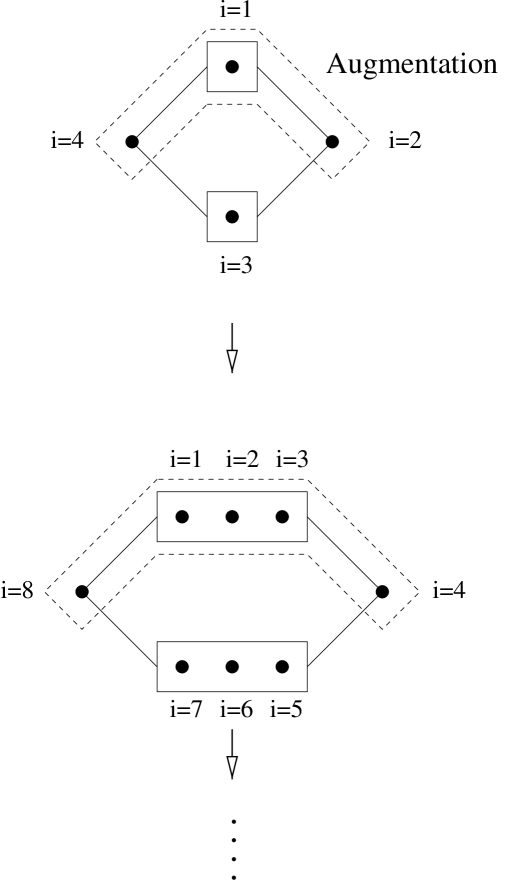
FIG. 6.: A DMRG iteration using periodic boundary conditions.

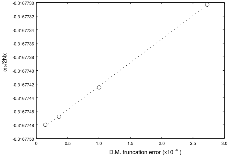
FIG. 7.: Dependence of the estimated ground state energy density $\omega_{0}/2Nx$ on the density matrix truncation eigenvalues, for $x=100$, $m/g=0.3$, $\theta=\pi$, using PBC.

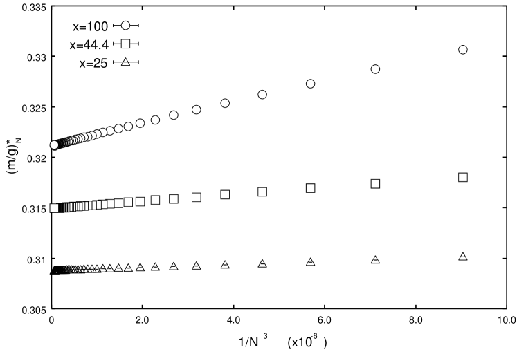
FIG. 8.: Pseudocritical points for various lattice spacings.

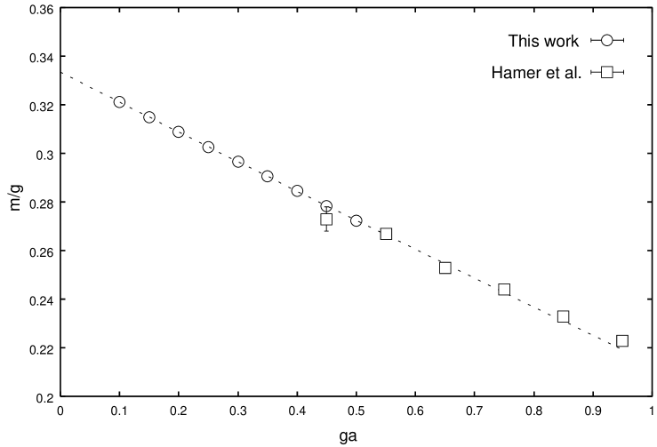
FIG. 9.: Critical line in the $m/g$ versus $1/\sqrt{x}=ga$ plane. Open circles are our present estimates, and squares are the previous results of Hamer et al. [13], which are in good agreement. The dashed line is a quadratic fit to the data in $ga$.

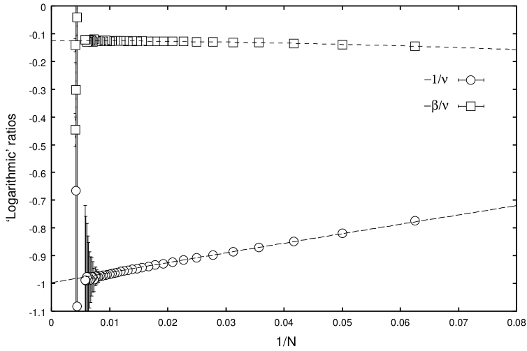
FIG. 10.: ‘Logarithmic’ ratio estimates of critical indices $-1/\nu$ and $-\beta/\nu$ for lattice spacing $1/\sqrt{x}=ga=0.45$. Quadratic fits in $1/N$ provide the bulk extrapolations. We estimate here $1/\nu=1.00(2)$ and $\beta/\nu=0.125(5)$.

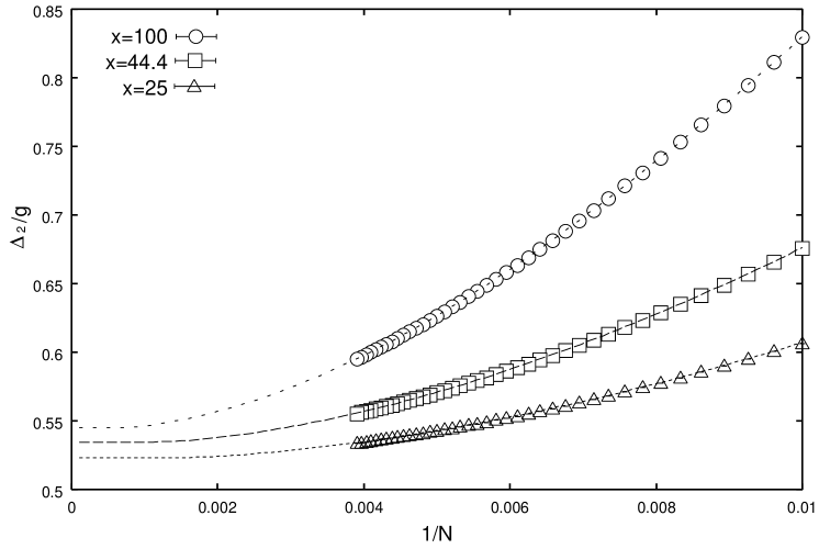
FIG. 11.: Bulk extrapolations for the 2-particle gap $\Delta_{2}/g$ for $m/g=0.0$ and $\theta=\pi$. Dashed lines are the fits to the data, according to (70)

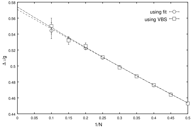
FIG. 12.: Continuum extrapolations for the 2-particle gap for $m/g=0.0$ and $\theta=\pi$. Data sets obtained through separate VBS and fit extrapolations.

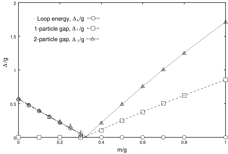
FIG. 13.: Final estimates for gaps in the 0-particle, 1-particle and 2-particle sectors at $\theta=\pi$. Dashed lines are merely to guide the eye.

FIG. 14.: The electric fields at either end of the chain in the presence of a single particle are $g/2,-g/2$ respectively. This precludes periodic boundary conditions due to the mismatch of electric fields.

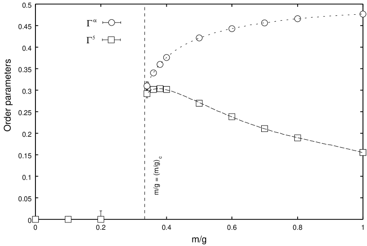
FIG. 15.: Order parameters $\Gamma^{\alpha}=\langle(L+\alpha)\rangle_{0}$, $\Gamma^{5}=\langle i\bar{\psi}\gamma_{5}\psi/g\rangle_{0}$ near the critical region. Dashed lines are merely to guide the eye.

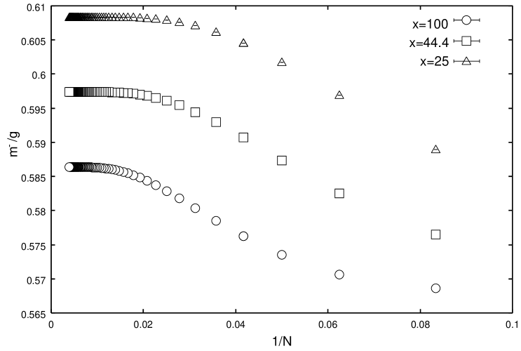
FIG. 16.: “Vector” mass gaps $m^{-}/g$ for $m/g=0$, finite lattices $N=10$-$256$, and various lattice spacings.

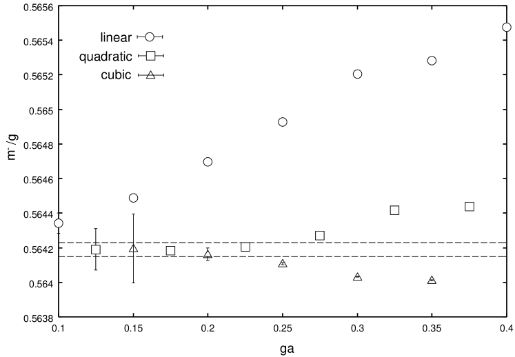
FIG. 17.: An example of our extrapolation procedure for the “vector” mass gaps at $m/g=0$. Circles, squares and triangles show linear, quadratic and cubic extrapolants respectively. Dashed lines show the upper and lower bounds for our final estimate. Here we estimate $m^{-}/g=0.56419(4)$.

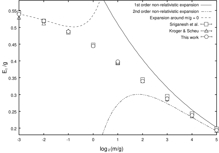
FIG. 18.: Comparison of our results for the “vector” state binding energies $E_{1}/g$ with other works. Squares mark the results of Sriganesh et al. [21] and triangles the results of Kröger and Scheu [30]. The results of Vary, Fields and Pirner [33] and Adam [34] were used for the expansion around $m/g=0$, while the non-relativistic expansions were done in the works of Hamer [36] and Sriganesh et al. [21].

REFERENCES

- [1] J. Schwinger, Phys. Rev. 128, 2425 (1962).
- [2] J. Lowenstein and J. Swieca, Ann. of Phys. 68, 172 (1971).
- [3] S. Coleman, R. Jackiw, and L. Susskind, Ann. of Phys. 93, 267 (1975).
- [4] A. Casher, J. Kogut, and L. Susskind, Phys. Rev. D 10, 732 (1974).
- [5] A. Casher, J. Kogut and L. Susskind, Ann. Phys. (N.Y.) 93, 267(1975).
- [6] S. Coleman, Ann. of Phys. 101, 239 (1976).
- [7] M. Creutz, Nucl. Phys. Proc. Suppl. 42, 56 (1995).
- [8] R. Narayanan, H. Neuberger and P. Vranis, Phys. Letts. B353, 507 (1995).
- [9] C. Gattringer, Phys. Rev. D53, 5090 (1996).
- [10] J. Kiskis and R. Narayanan, Phys. Rev. D62, 054501 (2000).
- [11] S.R. White, Phys. Rev. Lett. 69, 2863 (1992); Phys. Rev. B 48, 10345 (1993).
- [12] G.A. Gehring, R.J. Bursill and T. Xiang, Acta Phys. Pol. 91, 105 (1997).
- [13] C.J. Hamer, J. Kogut, D.P. Crewther, and M.M. Mazzolini, Nucl. Phys. B208, 413 (1982).
- [14] C.J. Burden and C.J. Hamer, Phys. Rev. D 37, 479 (1988), Appendix.
- [15] T. Banks, L. Susskind, and J. Kogut, Phys. Rev. D 13, 1043 (1976).
- [16] A. Carroll, J. Kogut, D.K. Sinclair, and L. Susskind, Phys. Rev. D 13, 2270 (1976).
- [17] F. Berruto, G. Grignani, G. W. Semenoff and P. Sodano, Phys. Rev. 57, 5070 (1998)
- [18] C.J. Hamer, Zheng Weihong and J. Oitmaa, Phys. Rev. D56, 55 (1997).
- [19] D.P. Crewther and C.J. Hamer, Nucl. Phys. B 170, 353 (1980).
- [20] A.C. Irving and A. Thomas, Nucl. Phys. B 215, 23 (1983).
- [21] P. Sriganesh, C.J. Hamer and R.J. Bursill, Phys. Rev. D 62, 034508 (2000).
- [22] O. Martin and S. Otto, Nucl. Phys. B203, 297 (1982)
- [23] A.J. Schiller and J. Ranft, Nucl. Phys. B225, 204 (1983)
- [24] S.R. Carson and R.D. Kenway, Ann. Phys. 166, 364 (1986).
- [25] C.F. Baillie, Nucl. Phys. B283, 217 (1987).
- [26] V. Azcoiti, G. Di Carlo, A. Galante, A.F. Grillo and V. Laliena, Phys. Rev. D50, 6994 (1994).
- [27] T. Eller, H.C. Pauli, and S.J. Brodsky, Phys. Rev. D 35, 1493 (1987).
- [28] H. Bergknoff, Nucl. Phys. B 122, 215(1977).
- [29] Y. Mo and R.J. Perry, J. Comput. Phys. 108, 159 (1993).
- [30] H. Kröger and N. Scheu, Phys. Lett. B 429, 58 (1998).
- [31] K. Melnikov and M. Weinstein, Phys. Rev. D62, 094504 (2000).
- [32] X-Y. Fang, D. Schütte, V. Wethkamp and A. Wichmann, Phys. Rev. D64, 014501 (2001).
- [33] J.P. Vary, T.J. Fields and H.J. Pirner, Phys. Rev. D 53, 7231(1996).
- [34] C. Adam, Phys. Lett. B 382, 383(1996); Ann. Phys.
- [35] K. Harada, A. Okazaki and M. Taniguchi, Phys. Rev. D 52, 2429 (1995); K. Harada, T. Heinzl and Christian Stern, Phys. Rev. D57, 2460 (1998)
- [36] C.J. Hamer, Nucl. Phys. B 121, 159(1977).
- [37] S. Mandelstam, Phys. Rev. D 11, 3026 (1975).
- [38] M.A. Martin-Delgado and G. Sierra, Phys. Rev. Letts. 83, 1514 (1999).
- [39] J. Kogut and L. Susskind, Phys. Rev. D 11, 395 (1975).
- [40] C.N. Yang, Phys. Rev. 85, 808 (1952); K. Uzelac and R. Jullien, J. Phys. A14, L151 (1981); C.J. Hamer, J. Phys. A15, L675 (1982).
- [41] M.N. Barber, in Phase Transitions and Critical Phenomena, vol. 8, edited by C. Domb and J. Lebowitz (Academic, New York, 1983).
- [42] C.J. Hamer and M.N. Barber, J. Phys. A 14, 241 (1981).
- [43] J.M. Vanden Broeck and L.W. Schwartz, SIAM (Soc. Ind. Appl. Math.) J. Math. Anal. 10, 658 (1979); M.N. Barber and C.J. Hamer, J. Aust. Math. Soc. B, Appl. Math. 23, 229 (1980).
- [44] E. Fradkin and L. Susskind, Phys. Rev. D17, 2637 (1978).
- [45] T. Schultz, D. Mattis and E. Lieb, Rev. Mod. Phys. 36, 856 (1964).