Light Hadron Masses in QCD with Valence Wilson Quarks at $\beta$=6.25 from a Parallel PC Cluster

Abstract

We present results for $\pi$, $\rho$ and proton and $\Delta$ masses from our recently built Pentium cluster. The previous results for quenched Wilson fermions by MILC and GF11 collaborations are compared at $\beta=6/g^{2}$=5.7 and 5.85 with the same parameters on the $8^{3}\times 32$ lattice. New data are shown at $\beta$=6.25 on the $12^{3}\times 36$ and $16^{3}\times 32$ lattices. Such a larger $\beta$ value is useful for extrapolating the lattice results to the continuum limit. The smearing technique is systematically investigated and shown to greatly improve the spectrum data.

Keywords: Hadron spectrum, Lattice QCD, Monte Carlo simulation on parallel computers

PACS: 11.15Ha, 12.38.Gc, 02.70.Lq

1 Introduction

The computational physics group[1] at the Zhongshan University is in a period of rapid development. The group’s interests[2, 3] cover such topics as lattice study of hadron spectroscopy[4, 5], glueball decay and mixing, QCD at finite density[6], quantum instontons[7] and quantum chaos[8] using the quantum action[9]. Most of these topics can be studied through Monte Carlo simulation, but can be quite costly in terms of computing power. In order to do large scale numerical investigations of these topics, we built a high performance parallel computer[10, 11] using PC components.

QCD has been accepted to be the most successful gauge theory of strongly interacting particles. Calculation of hadron spectroscopy remains to be an important task of non-perturbative studies of QCD using lattice methods. This paper is one of our first steps[3, 10] in the direction of studying hadron properties. Our reasons for performing simulations with Wilson valence quarks are twofold: First, we are interested in the analysis of hadronic spectroscopy for quenched Wilson fermions; Second, we are interested in exploring the performance of our cluster in actual lattice QCD simulations. We decided to do a spectrum calculation on the $8^{3}\times 32$ lattice at $\beta=5.7$ and 5.85, and on the $12^{3}\times 36$ and $16^{3}\times 32$ lattices at $\beta=6.25$. The results at smaller $\beta$ values are used to compare with those in the literature, while those at a larger $\beta$ value, corresponding to smaller lattice spacing $a$, are useful for extrapolating the lattice results to the continuum limit. The smearing technique is employed to improve the spectrum data. We hope our data will be an important addition to the lattice study of QCD spectrum.

The remainder of this paper is organized as follows. In Sect. 2, the basic ideas of lattice QCD with Wilson quarks are given. In Sect. 3, we describe the simulation parameters as well as some basic features of our cluster. In Sect. 4, we present new calculation of some light hadron masses. Finally, conclusions and outlook are given in Sect. 5.

2 Basic ideas of lattice QCD

Our starting point is the Wilson action [12]

$$S=-{\beta\over 6}\sum_{p}{\rm Tr}(U_{p}+U_{p}^{\dagger}-2)+\sum_{x,y}\bar{\psi}(x)M_{xy}\psi(y),$$ (1)

where $\beta=6/g^{2}$, and $U_{p}$ is the ordered product of gauge link variables $U_{\mu}(x)=e^{ig\int_{xa}^{xa+\hat{\mu}a}dx^{\prime}A_{\mu}(x^{\prime})}$ around an elementary plaquette. $a$ is the lattice spacing, $\hat{\mu}$ is the unit vector and $M$ is the fermionic matrix:

$$M_{xy}=\delta_{xy}-\kappa\sum_{\mu=1}^{4}\left[(1-\gamma_{\mu})U_{\mu}(x)\delta_{x,y-\hat{\mu}}+(1+\gamma_{\mu})U_{\mu}^{\dagger}(x-\hat{\mu})\delta_{x,y+\hat{\mu}}\right].$$ (2)

The fermion field $\psi$ on the lattice is related to the continuum one $\psi^{cont}$ by $\psi=\psi^{cont}\sqrt{a^{3}/(2\kappa)}$ with $\kappa=1/(2ma+8)$. Then all the physical quantities are calculable through Monte Carlo (MC) simulations with importance sampling. Fermion fields must be integrated out before the simulations, leading to the vacuum expectation value for an operator $F$

$$\langle F\rangle={\int[dU]\bar{F}([U])e^{-S_{g}([U])}\left(\det M\right)^{N_{f}}\over\int[dU]e^{-S_{g}([U])}\left(\det M\right)^{N_{f}}}\approx{1\over N_{\rm config}}\sum_{\mathcal{C}}\bar{F}[{\mathcal{C}}].$$ (3)

Here $N_{f}$ is the number of flavors, and $\bar{F}$ is the corresponding operator after Wick contraction of the fermion fields and the summation is over the gluonic configurations, ${\mathcal{C}}$, drawn from the Boltzmann distribution. In quenched approximation, $\det(M)=1$.

The correlation functions of a hadron is:

$$C_{h}(t)=\sum_{\vec{x}}\langle O_{h}^{\dagger}(\vec{x},t)O_{h}(\vec{0},0)\rangle,$$ (4)

where $O_{h}(\stackrel{{\scriptstyle\rightarrow}}{{x}},t)$ is a hadron operator. For sufficiently large values of $t$ and the lattice time period $T$, the correlation function is expected to approach the asymptotic form:

$$C_{h}(t)\rightarrow Z_{h}[\exp(-m_{h}at)+\exp(m_{h}at-m_{h}aT)].$$ (5)

Fitting the large $t$ behavior of the correlation function according to Eq. (5), the hadron mass $m_{h}$ is obtained.

3 Simulations

The quenched gauge field configurations and quark propagators were obtained using the recently built ZSU cluster[10, 11]. The full machine has 10 nodes, and each node consists of dual Pentium CPUs. The total internal memory is 1.28GB and the sustained speed is around 2 Gflops. An upgrade is planned. The cluster runs on the Linux operating system. To operate the cluster as a parallel computer, the programmer must design the algorithm so that it appropriately divides the task among the individual processors. We use MPI (Message Passing Interface), one of the most popular message passing standards.

We updated the pure SU(3) gauge fields with Cabibbo-Marinari quasi-heat bath algorithm[13], each iteration followed by 4 over-relaxation sweeps. The simulation parameters are listed in Tab. 1. The distance between two nearest stored configurations is 100. The auto-correlation time was computed to make sure that these configurations are independent.

The $u$ quark and $d$ quark are assumed to be degenerate. The quark propagators are calculated in the Coulomb gauge using the independent configurations mentioned above, and conjugate gradient for inversion of the Dirac matrix with preconditioning via ILU decomposition by checkerboards[14].

At $\beta=6.25$, we computed the $\pi$, $\rho$ and proton and $\Delta$ masses on the $12^{3}\times 36$ and $16^{3}\times 32$ lattices at four values of hopping parameter: $\kappa=0.1480$, 0.1486, 0.1492, and 0.1498 with point and smeared[17, 18] sources. In order to compare our results with those by MILC and GF11, the quenched simulations were also performed at $\beta=5.7$ and $\beta=5.85$ on the $8^{3}\times 32$ lattice. We repeated the quenched simulations of the MILC and GF11 collaborations, using the same set of $\kappa$ values [16, 17, 18] but on a $8^{3}\times 32$ lattice. Detailed data will be presented elsewhere [10].

4 Light hadron masses

To extract masses from the hadron propagators, we must average the correlation function of the hadron over the ensemble of gauge configurations, and use a fitting routine to evaluate the hadron masses $m_{h}$. We determined hadron masses by fitting our data under the assumption that there is a single particle in each channel [10].

Point source means a delta function, and smeared source means a spread-out distribution (an approximation to the actual wave-function of the quantum state). For example, the simplest operator for a meson is just $O_{h}(\stackrel{{\scriptstyle\rightarrow}}{{x}})={\bar{q}}(\vec{x})q(\vec{x})$, i.e. the product of quark and anti-quark fields at a single point. A disadvantage of this point source, is that this operator creates not only the lightest meson, but all possible excited states too. To write down an operator which creates more of the single state, one must “smear” the operator out, e.g. $\sum_{\vec{y}}~{}{\bar{q}}(\vec{x})f(\vec{x}-\vec{y})q(\vec{y})$ where $f(\vec{x})$ is some smooth function. Here we choose

$$f(\vec{x})=N\rm{exp}(-|\vec{x}|^{2}/r_{0}^{2}),$$ (6)

with $N$ a normalization factor. The size of the smeared operator should generally be comparable to the size of the hadron created. There is no automatic procedure [17] for tuning the smearing parameter $r_{0}$. One simply has to experiment with a couple of choices.

The effective meson mass for $\pi$ and $\rho$ as a function of time $t$ at $\beta=6.25$ and on the $16^{3}\times 32$ lattice is depicted in Figs. 1 and 2 respectively. As one sees, the plateau from which one can estimate the mass, is very narrow for point source, due to the reason mentioned above. When the smearing source is used, the width of the plateau changes with the smearing parameter $r_{0}$. We tried many values of $r_{0}$ and found that when $r_{0}>16$, the effective mass is almost independent on $r_{0}$ and the optimal value for $r_{0}$ is 26, where we observe the widest plateau.

The $\pi$, $\rho$, proton and $\Delta$ masses [10] at $\beta=5.7$ and on $8^{3}\times 32$ are consistent with the previous GF11 data [18] and those for the mesons at $\beta=5.85$ and on $8^{3}\times 32$ are comparable with those in [18] on the $16^{3}\times 32$ lattice. This means the finite size effects are very small. At $\beta=5.85$, we also see that our results for the proton and $\Delta$ masses[10] are bigger than the MILC data and consistent with the finite size behavior analysis in [17]. More detailed results will be given in [10]. In Fig. 3, we show the Edinburgh plot, ($m_{N}/m_{p}$) vs. ($m_{\pi}/m_{\rho}$) mass ratios.

In Figs. 4, and 5, we show respectively $(m_{\pi}a)^{2}$, $m_{\rho}a$, $m_{p}a$ and $m_{\Delta}a$ as a function of $1/\kappa$ at $\beta=6.25$ and on the $16^{3}\times 32$ lattice. Assuming that $(m_{\pi}a)^{2}$ is linear in $1/\kappa$, we can compute the critical coupling $\kappa_{c}$ at which the pion becomes massless. We extrapolate the data using:

$$(m_{\pi}a)^{2}=A\left({\frac{1}{\kappa}}-{\frac{1}{\kappa_{c}}}\right).$$ (7)

The results for $\kappa_{c}$, and $m_{\rho}a$, $m_{P}a$ and $m_{\Delta}a$ at $\kappa_{c}$ on the $12^{3}\times 36$ and $16^{3}\times 32$ are given in Tab.2, where the experimental value for the $\rho$ mass has been used as an input. The finite size effects are consistent with [17]. Also, the mass ratios $m_{P}/m_{\rho}$ and $m_{\Delta}/m_{\rho}$ seem to be closer the experimental values, 1.222 and 1.604 on the larger lattice. To compare $m_{P}$ and $m_{\Delta}$ with experiment, we need to do simulation on a larger lattice volume and carefully study the lattice spacing errors. In this aspect, it might be more efficient to use the improved action and some progress[20, 21] has been reported by some lattice groups in China.

5 Conclusions and Outlook

In this paper, we have presented new data on hadron masses in QCD with Wilson valence quarks at $\beta=6.25$ on the $12^{3}\times 36$ and $16^{3}\times 32$ lattices. Our results at $\beta=5.7$ are consistent and those at $\beta=5.85$ are comparable with the results in the literature. We have also made a more careful and systematic study of the smearing method. Such large scale simulations had usually required supercomputing resources [17, 18], but now they were all done on our recently built cluster for parallel computer. In the task of lattice QCD simulations, we are confident that ZSU’s Pentium cluster can provide a very flexible and extremely economical computing solution, which fits the demands and budget of a developing lattice field theory group. We are going to use the machine to produce more useful results of non-perturbative physics.

Acknowledgements

This work was in part based on the MILC collaboration’s public lattice gauge theory code. (See reference [19].) We are grateful to C. DeTar, C. McNeile, and D. Toussaint, for helpful discussions.

volume	$\beta$	warmup	stored configs.
$8^{3}\times 32$	5.7	200	200
$8^{3}\times 32$	5.85	200	200
$12^{3}\times 36$	6.25	200	200
$16^{3}\times 32$	6.25	600	600

Table 1: Simulation parameters

Lattice Volume	$12^{3}\times 36$	$16^{3}\times 32$
$\kappa_{c}$	0.1531(7)	0.1539(11)
$a(\kappa_{c})$	0.505(9) GeV-1	0.520(5) GeV-1
$m_{\pi}a(\kappa_{c})$	0.0	0.0
$m_{\rho}a(\kappa_{c})$	0.388(6)	0.399(8)
$m_{P}a(\kappa_{c})$	0.621(8)	0.611(5)
$m_{\Delta}a(\kappa_{c})$	0.770(3)	0.763(8)
$m_{P}/m_{\rho}$	1.598(4)	1.529(8)
$m_{\Delta}/m_{\rho}$	1.981(9)	1.908(9)

Table 2: Results of fitted $\kappa$, lattice spacing, and light hadron masses in the chiral limit at $\beta$=6.25.

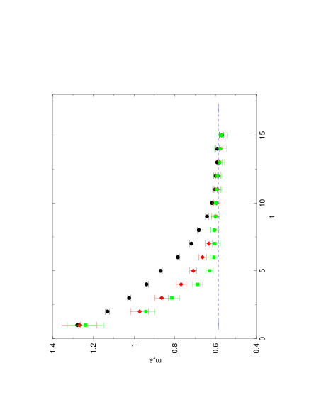
Figure 1: Pion effective mass fits to the correlation function at $\beta=6.25$ and $\kappa=0.1480$ and on the $16^{3}\times 32$ lattice. Data for the point source, smearing source for $r_{0}=8$, and $r_{0}=26$ are labelled by circles, diamonds, and squares respectively (from top to bottom).

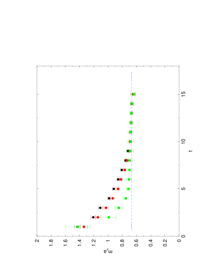
Figure 2: The meaning of the symbols are the same as Fig. 1, but the rho meson.

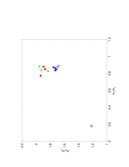
Figure 3: Edinburgh plot. Data are: simulations at $\beta=5.7$ (star), $\beta=5.85$ (filled circle) on the $8^{3}\times 32$ lattice, $\beta=6.25$ on the $12^{3}\times 36$ lattice (diamond) and $\beta=6.25$ on the $16^{3}\times 32$ lattice (filled square). The open square shows the real-world point.

Figure 4: Pion mass squared as a function of $1/\kappa$ for $\beta=6.25$ on the $16^{3}\times 32$ lattice. In this and the following figures, the error bars reflect the sum of statistical and systematic errors.

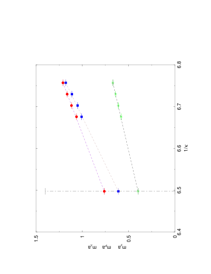
Figure 5: Rho, proton and Delta masses as a function of $1/\kappa$ for $\beta=6.25$ on the $16^{3}\times 32$ lattice. Results in the chiral limit (on the vertical dot-dashed line) are also shown.

References

- [1] Zhongshan University Computational group, http://qomolangma.zsu.edu.cn
- [2] X.Q. Luo and E.B. Gregory, editors, Non-Perturbative Methods and Lattice QCD, World Scientific, Singapore (2001), 308pp.
- [3] X.Q. Luo and E.B. Gregory, hep-lat/0011028.
- [4] X.Q. Luo and Q. Chen, Mod. Phys. Lett. A11 (1996) 2435.
- [5] X.Q. Luo, Q. Chen, S. Guo, X. Fang, and J. Liu, Nucl. Phys. B(Proc. Suppl.)53 (1997) 243.
- [6] E.B. Gregory, S. Guo, H. Kroger and X.Q. Luo, Phys. Rev. D62 (2000) 054508.
- [7] H. Jirari, H. Kroger, X.Q. Luo, K. Moriarty, and S. Rubin, Phys. Lett. A281 (2001) 1.
- [8] L. Caron, H. Jirari, H. Kroger, X.Q. Luo, G. Melkonyan, and K. Moriarty, Phys. Lett. A288 (2001) 145.
- [9] H. Jirari, H. Kroger, X.Q. Luo, K. Moriarty, and S. Rubin, Phys. Rev. Lett. 86 (2001) 187.
- [10] X.Q. Luo, E. Gregory, H. Xi, Z. Mei, J. Yang, Y. Wang, and Y. Lin, hep-lat/0107017.
- [11] X.Q. Luo, E. Gregory, H. Xi, J. Yang, Y. Wang, Y. Lin, and H. Ying, Nucl. Phys. B(Proc. Suppl.)106 (2002) 1046.
- [12] K.G. Wilson, Phys. Rev. D10 (1974) 2445; K.G.Wilson, in New Phenomena in Sub-nuclear Physics, Erice Lectures 1975, A. Zichichi, ed. (Plenum, New York, 1977).
- [13] N. Cabibbo and E. Marinari, Phys. Lett. B119 (1982) 387.
- [14] T. DeGrand, Comput. Phys. Commum. 52 (1988) 161.
- [15] SESAM-collaboration, Nucl. Phys. B(Proc. Suppl.)49 (1996) 386.
- [16] K.M. Bitar, et al, Phys. Rev. D46 (1992) 2169.
- [17] C. Bernard, et al., (MILC collaboration), Nucl. Phys. B(Proc. Suppl.)60A (1998) 3.
- [18] F. Bulter, H. Chen, J. Sexton, A. Vacarrino, and D. Weingarten, Nucl. Phys. B430 (1994) 179.
- [19] MILC Collaboration, http://physics.indiana.edu/sg/milc.html
- [20] D.Q. Liu, J.M. Wu, and Y. Chen, Chin. Phys. Lett. 18 (2001) 1442.
- [21] C. Liu and J. Ma, in [2], p65-p71; C. Liu, Chin. Phys. Lett. 18 (2001) 187.