Chiral symmetry restoration and the Z₃ sectors of QCD

Abstract

Quenched SU(3) lattice gauge theory shows three phase transitions, namely the chiral, the deconfinement and the Z₃ phase transition. Knowing whether or not the chiral and the deconfinement phase transition occur at the same temperature for all Z₃ sectors could be crucial to understand the underlying microscopic dynamics. We use the existence of a gap in the Dirac spectrum as an order parameter for the restoration of chiral symmetry. We find that the spectral gap opens up at the same critical temperature in all Z₃ sectors in contrast to earlier claims in the literature.

One of the most remarkable features of the QCD phase transition is the simultaneous vanishing of confinement and the restoration of chiral symmetry. Although there is much debate about the underlying mechanism which links the two transitions, their coincidence at a common critical temperature is considered a well established fact in lattice simulations (see e.g. [1] for a review). Interestingly, QCD in the quenched approximation has an additional Z₃ symmetry which allows us to obtain additional information. For pure gauge theory the phase transition can be described as spontaneous breaking of the Z₃ symmetry [2]. For temperatures larger than $T_{c}$ the Polyakov loop acquires a non-vanishing expectation value with a phase in one of the three sectors. Knowing whether the observed strict correlation between the chiral and deconfinement phase transitions persists in all Z₃ sectors could provide important clues for the understanding of confinement.

In [3] it was claimed on the basis of lattice calculations with staggered fermions, that the restoration of chiral symmetry happens at different temperatures in the real ($\varphi\sim 0$) and complex sector of the Polyakov loop ($\varphi\sim\pm 2\pi/3$). Several subsequent articles [4] analyzed possible mechanisms to explain this observation.

In this letter we reexamine this problem within lattice QCD using chirally improved fermions. In contrast to [3] we find that the critical $\beta$ of the chiral phase transition does not depend on the Z₃ sector, but is coincident with the Z₃ breaking transition in all three sectors.

Let us note that even if it were irrelevant for full QCD the center symmetry could still lead to fascinating phenomenological consequences in supersymmetric Yang-Mills theories [5]. Thus the investigation of its properties is also relevant on more general grounds.

Instead of directly measuring the chiral condensate we analyze in detail the spectrum of the lattice Dirac operator. The density $\rho(\lambda)$ of the eigenvalues $\lambda$ of the Dirac operator is connected to the chiral condensate via the Banks-Casher formula [6],

$$\langle\bar{\psi}\psi\rangle\;=\;-\frac{\pi}{V}\,\rho(0)\;,$$ (1)

where $\rho(0)$ is the eigenvalue density near the origin and $V$ is the volume of the box. Note that exact zero-modes which come from isolated instantons do not contribute to the density $\rho(0)$ at the origin. The reason is that the number of zero-modes is believed to scale as $V^{1/2}$ and thus they do not contribute when performing the thermodynamic limit in Eq. (1). At low temperatures when QCD is in the chirally broken phase the density is non-zero at the origin, while in the high temperature phase $\rho$ is zero in a finite region around the origin, i.e. the spectrum develops a gap (up to isolated zero modes) and the chiral condensate vanishes (compare Fig. 1 below). The question whether chiral symmetry is restored at the same critical temperature in all sectors of the Polyakov loop can now be reformulated in terms of the spectral gap: As we increase the temperature, does the gap open up at the same temperature for all three sectors of the Polyakov loop?

Before the advent of chirally symmetric formulations for the lattice Dirac operator such a study was quite awkward. In particular the spectrum of the Wilson lattice Dirac operator shows large fluctuations close to the origin [7] and the notion of a spectral density is not well defined. The situation has changed, since the re-discovery of the Ginsparg-Wilson equation [8]. Dirac operators $D$ which obey the Ginsparg-Wilson equation have eigenvalues which lie on a circle and it is straightforward to identify a spectral density and study the emergence of the spectral gap. However, the only exact solution of the Ginsparg-Wilson equation, the overlap operator [9], has the drawback of being very expensive in a numerical implementation.

Here we work with the chirally improved operator which is a systematic expansion of a solution of the Ginsparg-Wilson equation [10]. In particular we use an approximation which has 19 terms in the expansion and is described in detail in [11]. The computation of the eigenvalues of the Dirac operator was done with the implicitly restarted Arnoldi method [12].

For our quenched gauge configurations we use the Lüscher-Weisz action [13]. We work on lattices of size $L_{T}\times L^{3}$ with the temporal extent $L_{T}=6$ and two values for the spatial extent, $L=16$ and $L=20$. We use periodic boundary conditions for the gauge fields, while for the fermions the boundary conditions are periodic only for the space directions but anti-periodic for the time direction. Our statistics is 800 configurations for the $6\times 16^{3}$ lattices and 400 for the $6\times 20^{3}$ lattices. We use 6 different values of the inverse coupling $\beta$ which gives rise to ensembles on both sides of the phase transition. In Table I we list our values of $\beta$, the lattice spacing $a$ [14] and the temperature $T$. We used the coefficients given by tadpole-improved perturbation theory [13, 15]. Our values for the couplings $\beta_{rt}$ and $\beta_{pg}$ for the rectangle and parallelogram terms in the Lüscher-Weisz action can be found in [14].

$\beta$	8.10	8.20	8.25	8.30	8.45	8.60
$a\;$ [fm]	0.125	0.115	0.110	0.106	0.094	0.084
$T\;$ [MeV]	264	287	299	311	350	391

TABLE I.: Parameters for our gauge field configurations. We list the values of $\beta$, the lattice spacing $a$ and the temperature $T$.

Let us begin the discussion of the spectral gap with a look at typical spectra of our Dirac operator. In Fig. 1 we show the distribution in the complex plane of the 50 smallest eigenvalues $\lambda$ for three different gauge configurations on $6\times 20^{3}$ lattices. The symbols are our numerical results and the full curve is the so-called Ginsparg-Wilson circle, i.e. the circle of radius 1 in the complex plane with center 1. For our approximate Ginsparg-Wilson operator the eigenvalues do not fall exactly on the circle but show small fluctuations around the circle. However, the eigenvalues are sufficiently well ordered to allow for the notion of a spectral density and a clear identification of the spectral gap.

The plot on the left-hand side shows the spectrum for a configuration in the low temperature, chirally broken phase. For this case the eigenvalues extend all the way to the origin and there is a non-vanishing $\rho(0)$ such that the Banks-Casher relation (1) gives rise to a non-vanishing chiral condensate.

The central and the right-hand side plots show spectra for configurations in the high-temperature, chirally symmetric phase. The central plot is for a configuration with complex Polyakov loop $P$, while the right-hand side result is for real Polyakov loop. Both of these plots have a well pronounced spectral gap. The spectral density at the origin vanishes and so does the chiral condensate. For the complex sector the gap is considerably smaller than for the real sector.

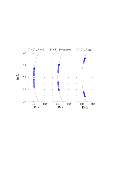
FIG. 1.: Three typical spectra of the chirally improved operator. Only the 50 eigenvalues closest to the origin are plotted: Left plot: the chirally broken phase ($6\times 20^{3},\beta=8.10$); Central plot: the symmetric phase ($6\times 20^{3},\beta=8.60$) for complex Polyakov loop; Right plot: the symmetric phase for real Polyakov loop. The full curve is the Ginsparg-Wilson circle.

One can understand this difference between the sectors by considering the fermion boundary conditions. In the real sector the boundary condition

$$\psi(\vec{x},t+1/T)\;=\;-\,\psi(\vec{x},t)$$ (2)

gives a Matsubara frequency $\pi T$ to the fermions. In the complex Z₃ sectors the boundary condition is effectively

$$\psi(\vec{x},t+1/T)\;=\;e^{\pm i\pi/3}\psi(\vec{x},t),$$ (3)

giving a Matsubara frequency $\pi T/3$. In the free-field case (i.e. $\beta\to\infty$) the smallest eigenvalue is equal to the Matsubara frequency, giving a gap 3 times larger in the case of (2) compared with (3). It is thus reasonable that the real sector gap is considerably larger than the complex sector gap in the interacting case too.

In quenched QCD the finite temperature phase transition appears to be a weak first order phase transition [16]. A first order phase transition is governed by the mixing of two phases and the behavior of their free energies. In our particular example we have a low temperature phase characterized by a vanishing spectral gap and a high temperature phase with a finite spectral gap. For temperatures sufficiently below or above the critical temperature the system is in only one of the two phases while near the critical temperature the system shows mixing of the two phases.

We demonstrate this mixing in Fig. 2 where we show histograms for the distribution of the spectral gap at three different values of the temperature. We define the spectral gap $g_{\lambda}$ to be the imaginary part of the smallest eigenvalue which is not a zero-mode (as remarked above, zero-modes do not contribute to the spectral density). Zero-modes can be identified uniquely since for our chirally improved operator it can be shown that they have exactly vanishing imaginary part and the corresponding eigenstates have a non-vanishing matrix element with $\gamma_{5}$, while this matrix element vanishes identically for non-zero-modes.

We show histograms for the distribution of $g_{\lambda}$ for $T<T_{c},T\sim T_{c}$ and for $T>T_{c}$. The top row displays the results for the complex sector of the Polyakov loop $P$, while the bottom row is for real Polkyakov loop. The data were computed on $6\times 20^{3}$ lattices. Since for the real sector ($\varphi\sim 0$) the statistics is only half of the statistics for the complex sector ($\varphi\sim+2\pi/3$ and $-2\pi/3$) we doubled the bin size for the two histograms in the real sector at $T\sim T_{c}$ and $T>T_{c}$.

FIG. 2.: Histograms for the spectral gap $ag_{\lambda}$. We show our results for lattice size $6\times 20^{3}$ at three temperatures $T<T_{c}$ ($\beta=8.10$), $T\sim T_{c}$ ($\beta=8.30$) and $T>T_{c}$ ($\beta=8.60$). The top row displays the results for the complex sector of the Polyakov loop $P$, while the bottom row is for real Polyakov loop.

At $T<T_{c}$ we find for all sectors a single peak near the origin. This peak is not located exactly at 0 since also in the chirally broken phase the Dirac operator of a finite system has a microscopical gap which vanishes as $L^{-3}$ [17]. For temperatures near $T_{c}$ the histograms show a clear double peak structure characteristic for the first order transition. The left peak corresponds to the chirally broken phase with a vanishing gap and the right peak is from the chirally symmetric phase with non-vanishing gap. As one increases the temperature further, only the right peak survives. As already noted in the discussion of Fig. 1 the gap is larger in the real sector, i.e. the right peak sits at larger values of $g_{\lambda}$ for the real sector. In addition this peak is wider than the corresponding peak in the complex sector, i.e. the gap fluctuates more strongly around its mean value in the real sector.

In order to describe the first order transition we use a simple ansatz for the behavior of observables. Let us first discuss the somewhat simpler case of the Polyakov loop. In an infinite system the Polyakov loop $P$ vanishes below $\beta_{c}$ and has a non-vanishing modulus $|P|$ above $\beta_{c}$. On a finite lattice the Polyakov loop does not vanish exactly below $\beta_{c}$ but disappears like $V^{-1/2}$, i.e. like $cL^{-3/2}$ with some constant $c$. Above $\beta_{c}$ the dependence on $L$ is negligible and to leading order $P$ is linear in $\beta$, i.e. described by $d+k(\beta-\beta_{c})$. Following the ideas in [18] one arrives at the conclusion that near the transition the expectation value of the modulus of the Polyakov loop should be given by:

$$\langle|P|\rangle=\frac{cL^{-3/2}\,e^{-\Delta fL^{3}(\beta-\beta_{c})}\,+\,3[d+k(\beta-\beta_{c})]}{e^{-\Delta fL^{3}(\beta-\beta_{c})}\;+\;3}\;.$$ (4)

The term $-\Delta fV(\beta-\beta_{c})$ is the difference in the free energies of the two phases. At $\beta=\beta_{c}$ the two free energies are equal while below $\beta_{c}$ the free energy of the chirally broken phase is smaller than the free energy of the chirally symmetric phase and vice-versa above $\beta_{c}$. The factors 3 in the second terms in the numerator and denominator come from the three possible values for the phase of the Polyakov loop.

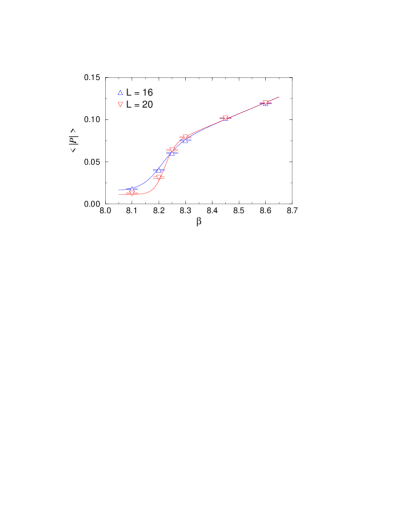
FIG. 3.: The expectation value $\langle|P|\rangle$ of the modulus of the Polyakov loop as a function of $\beta$. The symbols indicate the numerical results while the full curve is a fit to Formula (4). We display results for $6\times 16^{3}$ and $6\times 20^{3}$ lattices.

In Fig. 3 we show a fit of Formula (4) (full curves) to our numerical data (symbols). In particular we present a common fit to both the $6\times 16^{3}$ and $6\times 20^{3}$ ensembles. This is possible since the parameters $d$ and $k$ are essentially independent of $L$. The fit result for $\beta_{c}$ is given in Table II below. The fit demonstrates that both the $L$ and the $\beta$ dependence are well described by Formula (4).

For the expectation value of the spectral gap $g_{\lambda}$ we use a similar ansatz.

$$\langle g_{\lambda}\rangle_{r,c}\;=$$ (5)

$$\frac{c^{\prime}L^{-3}\,e^{-\Delta fL^{3}(\beta-\beta_{c})}\,+\,3[d_{r,c}(L)+k_{r,c}(L)(\beta-\beta_{c})]}{e^{-\Delta fL^{3}(\beta-\beta_{c})}\,+\,3}.$$ (6)

The subscripts $r$ and $c$ indicate the real respectively complex sectors of the Polyakov loop. Note that now we use the known $L^{-3}$ behavior of the microscopical spectral gap in the chirally broken phase [17]. In the chirally symmetric phase the gap is essentially linear in $\beta$ but the coefficients $d_{r,c}$ and $k_{r,c}$ turn out to be $L$-dependent. Thus in a common fit to the $6\times 16^{3}$ and $6\times 20^{3}$ ensembles these parameters had to be varied independently. Again the fit results for $\beta_{c}$ are given in Table II. In Fig. 4 we plot our numerical data for the gap together with the curves (5). The top plot gives the results for the complex sector while the bottom plot shows the real sector. As for the Polyakov loop we find that the numerical data are reasonably well described by the simple first order transition formula.

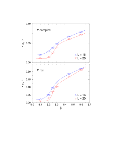
FIG. 4.: The spectral gap in lattice units as a function of $\beta$. The symbols indicate the numerical results and the full curve is a fit to Formula (5). We display results for $6\times 16^{3}$ and $6\times 20^{3}$.

When comparing the results for the critical beta as given in Table II we find that within the accuracy we achieved the spectral gap vanishes at the same $\beta_{c}$ for both the real and the complex sectors of the Polyakov loop. Furthermore this value is compatible with $\beta_{c}$ as obtained from the analysis of the Polyakov loop. Combining the three methods we find a critical temperature of $300\pm 3$ MeV for the Lüscher-Weisz action which is slightly larger than the result for Wilson’s gauge action.

Measurement :	$\langle|P|\rangle$	$\langle g_{\lambda}\rangle_{complex}$	$\langle g_{\lambda}\rangle_{real}$
$\beta_{c}$ :	8.24(1)	8.29(2)	8.27(2)
$T_{c}$ [MeV] :	296(3)	308(5)	303(5)

TABLE II.: Values of $\beta_{c}$ and the critical temperature from the analysis of the Polyakov loop and the spectral gap in the complex and the real sectors for the ensembles with Lüscher-Weisz action and chirally improved fermions.

Acknowledgements: The numerical calculations were done on the Hitachi SR8000 of the Leibniz Rechenzentrum in Munich. We thank the staff of the LRZ for training and support. C. Gattringer acknowledges support by the Austrian Academy of sciences (APART 654).

REFERENCES

- [1] F. Karsch, Lattice QCD at high temperature and density, hep-lat/0106019.
- [2] A. M. Polyakov, Phys. Lett. 72B, 477 (1978); B. Svetitsky and L.G. Yaffe, Nucl. Phys. B210 [FS6], 423 (1982).
- [3] S. Chandrasekharan and N.H. Christ, Nucl. Phys. Proc. Suppl. 47 (1996) 527.
- [4] P.N. Meisinger and M.C. Ogilvie, Phys. Lett. B 379 (1996) 163; S. Chandrasekharan and S. Huang, Phys. Rev. D 53 (1996) 5100; M.A. Stephanov, Phys. Lett. B 375 (1996) 249.
- [5] A. Campos, K. Holland, and U.J. Wiese, Phys. Rev. Lett. 81 (1998) 2420 ; K. Holland and U.J. Wiese; In Shifman, M. (ed.): At the frontier of particle physics, vol. 3, hep-ph/0011193.
- [6] T. Banks and A. Casher, Nucl. Phys. B169 (1980) 103.
- [7] C. Gattringer and I. Hip, Nucl. Phys. B 541 (1999) 305, Nucl. Phys. B 536 (1998) 363.
- [8] P.H. Ginsparg and K.G. Wilson, Phys. Rev. D 25 (1982) 2649.
- [9] R. Narayanan and H. Neuberger, Phys. Lett. B 302 (1993) 62, Nucl. Phys. B 443 (1995) 305.
- [10] C. Gattringer, Phys. Rev. D 63 (2001) 114501.
- [11] C. Gattringer, I. Hip and C.B. Lang, Nucl. Phys. B597 (2001) 451; C. Gattringer, M. Göckeler, P.E.L. Rakow, S. Schaefer and A. Schäfer, Nucl. Phys. B 618 (2001) 205.
- [12] D. C. Sorensen, SIAM J. Matrix Anal. Appl. 13 (1992) 357; R. B. Lehoucq, D. C. Sorensen and C. Yang, ARPACK User’s Guide, SIAM, New York, 1998.
- [13] M. Lüscher and P. Weisz, Commun. Math. Phys. 97 (1985) 59; Erratum: 98 (1985) 433; G. Curci, P. Menotti and G. Paffuti, Phys. Lett. B 130 (1983) 205, Erratum: B 135 (1984) 516.
- [14] C. Gattringer, R. Hoffmann, S. Schaefer, hep-lat/0112024.
- [15] M. Alford, W. Dimm, G.P. Lepage, G. Hockney and P.B. Mackenzie, Phys. Lett. B 361 (1995) 87; G.P. Lepage and P.B. Mackenzie, Phys. Rev. D 48 (1993) 2250; J. Snippe, Nucl. Phys. B 498 (1997) 347.
- [16] G. Boyd, J. Engels, F. Karsch, E. Laermann, C. Legeland, M. Lütgemeier and B. Petersson, Nucl. Phys. B469 (1996) 419.
- [17] J.J.M. Verbaarschot and T. Wettig, Ann. Rev. Nucl. Part. Sci. 50 (2000) 343.
- [18] C. Borgs and R. Koteck, Phys. Rev. Lett. 68 (1992) 1734; C. Borgs and W. Jahnke, Phys. Rev. Lett. 68 (1992) 1738.