Monopoles in Lattice QCD with Abelian Projection as Quantum Monopoles

Abstract

Within the context of the Abelian Projection of QCD monopole-like quantum excitations of gauge fields are studied. We start with certain classical solutions, of the SU(2) Yang-Mills field equations, which are not monopole-like and whose energy density diverges as $r\rightarrow\infty$. These divergent classical solutions are then quantized using a modified version of Heisenberg’s quantization technique for strongly interacting, nonlinear fields. The modified Heisenberg quantization technique leads to a system of equations with mixed quantum and classical degrees of freedom. By applying a Feynman path integration over the quantum degrees of freedom the quantum-averaged solution gives a nondivergent, monopole-like configuration after Abelian Projection.

I Introduction

Monopoles have been studied within both Abelian dirac and non-Abelian thooft gauge theories. Usually one starts with a classical monopole configuration (i.e. having a magnetic field which becomes Coulombic as $r\rightarrow\infty$) and then consider the quantum corrections to the system. One difficulty with this approach is that the coupling strength of monopole configurations is large due to the Dirac quantization condition dirac which requires that there be an inverse relationship between electric and magnetic couplings. A perturbatively small electric coupling requires a non-perturbatively large magnetic coupling. The perturbative quantization techniques do not work well with monopoles for the same reason that they have trouble with QCD in the low energy regime : the couplings are non-perturbatively large.

Numerical simulations in lattice QCD show that the configurations of gauge fields with monopoles dominate in the path integral, i.e. monopole configurations are important contributors to the QCD string tension. Thus the expectation value of any physical quantity $\langle\Upsilon\rangle$ in non-Abelian gauge theory can be accurately calculated (see for review Ref. pol ) in terms of the monopole currents extracted from the projected Abelian fields. Magnetic monopoles necessarily emerge as relevant degrees of freedom in the Abelian Projections of lattice gluodynamics. In this paper we present a specific picture of how such magnetic monopole configurations can emerge and dominate the QCD path integral. We start with spherically symmetric classical solutions to the SU(2) field equations. These solutions have a divergent energy density. However in constrast to the Wu-Yang monopole solutions, which are divergent due to fields that blow up at $r=0$, our solutions are divergent due to fields which blow up at $r=\infty$. These divergent solutions are parameterized by two ansatz functions. One of the ansatz functions smoothly and monotonically diverges at $\infty$ while the other functions strongly oscillates. Applying a modified variant of a non-perturbative quantization method originally used by Heisenberg hs1 hs3 , we find that the quantized version of our divergent classical solution becomes well behaved: the divergent ansatz function now goes to $0$ at $\infty$, and the rapid ocsillations of the other ansatz function are “smoothed” out. Rather than quantizing an SU(2) field configuration which is monopole-like already at the classical level, we quantized (using Heisenberg’s method) a non-monopole configuration, which has fields and an energy density which diverge at spacial infinity ($r\rightarrow\infty$). After quantization this classically divergent solution becomes physically well behaved, and its asymptotic magnetic field becomes monopole-like. This may indicate that monopoles are inherently quantum objects: rather than quantizing a configuration which is monopole-like at the classical level, real monopoles might arise as a consequence of quantizing non-monopole classical solutions.

II Classical SU(2) solution

In this section we will briefly review the classical, spherically symmetric, SU(2) Yang-Mills theory solutions to which we will apply the modified Heisenberg quantization method. We begin with the following ansatz for pure SU(2) Yang-Mills theory

$$A^{a}_{0} = \frac{x^{a}}{r^{2}}g(r),$$ (1)

$$A^{a}_{i} = \epsilon_{aij}\frac{x^{j}}{r^{2}}\left[1-f(r)\right],$$ (2)

here $a=1,2,3$ is a color index; the Latin indices $i,j,k,l=1,2,3$ are space indices. This is the Wu-Yang ansatz wu .

Under this ansatz the Yang - Mills equations ($D^{\mu}{F^{a}}_{\mu\nu}=0$) become

$$r^{2}f^{\prime\prime} = f^{3}-f-fg^{2},$$ (3)

$$r^{2}g^{\prime\prime} = 2gf^{2}$$ (4)

where the primes indicate differentiation with respect to $r$. In the asymptotic limit $r\rightarrow\infty$ the general solution to Eqs. (3), (4) approaches the form

$$f(x) \approx A\sin\left(x^{\alpha}+\phi_{0}\right),$$ (5)

$$g(x) \approx \alpha x^{\alpha}+\frac{\alpha-1}{4}\frac{\cos{\left(2x^{\alpha}+2\phi_{0}\right)}}{x^{\alpha}},$$ (6)

$$A^{2} = \alpha(\alpha-1)$$ (7)

where $x=r/r_{0}$ is a dimensionless radius and $r_{0},\phi_{0}$, and $A$ are constants. The plot of these functions are presented on the Fig.1, 2.

Figure 1: Function $f(x)$

Figure 2: Function $g(x)$

The numerical study of Eqs. (3), (4) showed that the approximate form of the solution in Eqs. (5) - (7) was a good representation even for $r$ close to the origin. These solutions can be compared with the certain confining potentials used in phenomenological studies of quarkonia bound states eich . It is possible to find analytic solutions with increasing gauge potentials, similar to the above numerical solution for the ansatz $g(x)$, if one couples the Yang-Mills fields to a scalar field yos . However, it is the increasing of $g(r)$ that leads to the field energy and action of this solution diverging as $r\rightarrow\infty$.

The “magnetic” ($H_{i}^{a}=\epsilon_{ijk}F^{a}_{jk}$) and “electric” ($E_{i}^{a}=F^{a}_{0i}$) fields associated with this solution can be found from the non-Abelian gauge potentials, $A_{\mu}^{a}$, and have the following behavior

$$H^{a}_{r} \propto \frac{f^{2}-1}{r^{2}}, \qquad H^{a}_{\varphi}\propto f^{\prime}, \qquad H^{a}_{\theta}\propto f^{\prime},$$ (8)

$$E^{a}_{r} \propto \frac{rg^{\prime}-g}{r^{2}}, \qquad E^{a}_{\varphi}\propto\frac{fg}{r}, \qquad E^{a}_{\theta}\propto\frac{fg}{r}.$$ (9)

III Extraction of the off-diagonal components of gauge potential

Our SU(2) gauge potential (1) (2) can be written as

$$A^{a}_{\theta} = \left[1-f(r)\right]\left\{\sin\varphi;-\cos\varphi;0\right\},$$ (10)

$$A^{q}_{\varphi} = \left[1-f(r)\right]\sin\theta\left\{\cos\theta\cos\varphi;\cos\theta\sin\varphi;-\sin\theta\right\},$$ (11)

$$A^{a}_{t} = \frac{g(r)}{r}\left\{\sin\theta\cos\varphi;\sin\theta\sin\varphi;\cos\theta\right\}.$$ (12)

The gauge transformation

$${A^{\prime}}^{a}_{\mu}=S^{-1}A^{a}_{\mu}S-i\left(\partial_{\mu}S^{-1}\right)S$$ (13)

with the matrix

$$S=\begin{pmatrix}\cos\frac{\theta}{2}&-e^{-i\varphi}\sin\frac{\theta}{2}\\ e^{i\varphi}\sin\frac{\theta}{2}&\cos\frac{\theta}{2}\end{pmatrix}$$ (14)

leads to the following result

$$A^{\prime}_{\theta} = f(r)\begin{pmatrix}0&-ie^{-i\varphi}\\ ie^{i\varphi}&0\end{pmatrix},$$ (15)

$$A^{\prime}_{\varphi} = \left(\cos\theta-1\right)\begin{pmatrix}1&0\\ 0&-1\end{pmatrix}-f(r)\sin\theta\begin{pmatrix}0&e^{-i\varphi}\\ e^{i\varphi}&0\end{pmatrix},$$ (16)

$$A^{\prime}_{t} = \frac{g(r)}{r}\begin{pmatrix}1&0\\ 0&-1\end{pmatrix}.$$ (17)

In this form we see that if $f(r)\rightarrow 0$ as $r\rightarrow\infty$ then only the first term in Eq. (16) is relevant. This first term is in the U(1) subgroup of the SU(2) gauge field, and gives rise to a magnetic monopole.

Under the assumption (originally found in ref. thooft2 ) that the U(1) diagonal components of the non-Abelian gauge field are the most important for confinement, one tries to make a gauge choice which minimizes or excludes the off-diagonal components of the gauge potential (i.e. the Cartan subalgebra). For example, in Maximal Abelian Projection kronfeld , kondo the following gauge condition is applied

$$D_{\mu}\left(A^{H}\right)A^{off}_{\mu}=\partial_{\mu}A^{off}_{\mu}+ig\left[A^{H}_{\mu},A^{off}_{\mu}\right]=0$$ (18)

where $A_{\mu}=A^{H}_{\mu}+A^{off}_{\mu}$. $A^{H}_{\mu}$ is the Abelian, diagonal pomponent of $A_{\mu}$ while $A^{off}_{\mu}$ are the off-diagonal components of $A_{\mu}$. This gauge corresponds to the minimization of the following functional pol

$$R=\int\left\{\left[A^{1}_{\mu}\right]^{2}+\left[A^{2}_{\mu}\right]^{2}\right\}d^{4}x$$ (19)

where $A^{off}_{\mu}=A^{1,2}_{\mu}$. Lattice calculations (for review, see for example, pol2 ) indicate that monopole-like gauge field configurations are dominate in the path integral. Here we show that one can reach this same conclusion by using a variant of Heisenberg’s quantization method on non-monopole, classical solution. By quantizing the non-Abelian we find that $f(r)\rightarrow 0$ as $r\rightarrow\infty$. Thus the quantized non-Abelian fields asymptotically appear as monopoles.

IV Heisenberg’s Non-Perturbative Quantization

Although the confining behavior of these classical solutions is interesting due to their similarity with certain phenomenological, confining potentials, the infinite field energy makes their physical importance/meaning uncertain. One possible resolution to the divergent field energy is if quantum effects removed the bad long distance behavior. The difficulty is that strongly interacting, nonlinear theories are notoriously hard to quantize. In order to take into account the quantum effects on these solutions we will employ a variation of the method used by Heisenberg hs1 in attempts to quantize the nonlinear Dirac equation. It can be shown dzh4 that the Gor’kov’s equations (and consequently the Ginzburg - Landau equations) in superconductivity theory is the direct application of Heisenberg’s idea for quantization of Cooper pairs in the superconductor. We will outline the key points of the method by using the nonlinear Dirac equation as an illustrative example. The nonlinear spinor field equation considered by Heisenberg had the following form :

$$\gamma^{\mu}\partial_{\mu}{\hat{\psi}(x)}-l^{2}\Im[{\hat{\psi}}({\hat{\bar{\psi}}}\psi)]=0$$ (20)

where $\gamma^{\mu}$ are Dirac matrices; ${\hat{\psi}(x)},{\hat{\bar{\psi}}}$ are the spinor field and its adjoint respectively; $\Im[{\hat{\psi}}({\hat{\bar{\psi}}}{\hat{\psi}})]$ is the general nonlinear spinor self interaction term which involved three spinor fields and various combinations of $\gamma^{\mu}$’s and/or $\gamma^{5}$’s. The constant $l$ has units of length, and sets the scale for the strength of the interaction. Next one defines $\tau$ functions as

$$\tau(x_{1}x_{2}...|y_{1}y_{2}...)=\langle 0|T[{\hat{\psi}}(x_{1}){\hat{\psi}}(x_{2})...{\hat{\psi}}^{\ast}(y_{1}){\hat{\psi}}^{\ast}(y_{2})...]|\Phi\rangle$$ (21)

where $T$ is the time ordering operator; $|\Phi\rangle$ is a state for the system described by Eq. (20). Applying Eq. (20) to (21) we obtain the following infinite system of equations for various $\tau$’s

$$l^{-2}\gamma^{\mu}_{(r)}\frac{\partial}{\partial x^{\mu}_{(r)}} \tau(x_{1}...x_{n}|y_{1}...y_{n})=\Im[\tau(x_{1}...x_{n}x_{r}|y_{1}...y_{n}y_{r})]+$$ (22)

$$\delta(x_{r}-y_{1})\tau(x_{1}...x_{r-1}x_{r+1}...x_{n}|y_{2}...y_{r-1}y_{r+1}...y_{n})+$$

$$\delta(x_{r}-y_{2})\tau(x_{1}...x_{r-1}x_{r+1}...x_{n}|y_{1}y_{2}...y_{r-1}y_{r+1}...y_{n})+...$$

Eq. (22) represents one of an infinite set of coupled equations which relate various order (given by the index $n$) of the $\tau$ functions to one another. To make some head way toward solving this infinite set of equations Heisenberg employed the Tamm-Dankoff method whereby he only considered $\tau$ functions up to a certain order. This effectively turned the infinite set of coupled equations into a finite set of coupled equations.

For the SU(2) Yang-Mills theory this idea leads to the following Yang-Mills equations for the quantized SU(2) gauge field

$$D_{\mu}\hat{F}^{a\mu\nu}=0$$ (23)

here $\hat{F}^{a\mu\nu}$ is the field operator of the SU(2) gauge field.

One can show that Heisenberg’s method is equivalent to the Dyson-Schwinger system of equations for small coupling constants. One can also make a comparison between the Heisenberg method and the standard Feynman diagram technique. With the Feynman diagram method quantum corrections to physical quantities are given in terms of an infinite number of higher order, loop diagrams. In practice one takes only a finite number of diagrams into account when calculating the quantum correction to some physical quantity. This standard diagrammatic method requires a small expansion parameter (the coupling constant), and thus does not work for strongly coupled theories. The Heisenberg method was intended for strongly coupled, nonlinear theories, and we will apply a variation of this method to the classical solution discussed in the last section.

We will consider a variation of Heisenberg’s quantization method for the present non-Abelian equations by making the following assumptions dzh2 :

1. The physical degrees of freedom relevant for studying the above classical solution (which after quantization will be spherically symmetric excitations in QCD vacuum) are given entirely by the two ansatz functions $f,g$ appearing in Eqs. (3), (4). No other degrees of freedom will arise through the quantization process.

2. From Eqs. (5), (6) we see that one function $f(r)$ is a smoothly varying function for large $r$, while another function, $g(r)$, is strongly oscillating. Thus we take $g(r)$ to be an almost classical degree of freedom while $f(r)$ is treated as a fully quantum mechanical degree of freedom. Naively one might expect that only the behavior of second function would change while the first function stayed the same. However since both functions are interrelated through the nonlinear nature of the field equations we find that both functions are modified.

To begin we replace the ansatz functions by operators ${\hat{f}}(x),{\hat{g}}(x)$.

$$r^{2}{\hat{f}}^{\prime\prime} = {\hat{f}}^{3}-{\hat{f}}-{\hat{f}}{\hat{g}}^{2},$$ (24)

$$r^{2}{\hat{g}}^{\prime\prime} = 2{\hat{g}}{\hat{f}}^{2}$$ (25)

These equations can be seen as an approximation of the quantized SU(2) Yang-Mills field equations (23). Taking into account assumption (2) we let ${\hat{g}}\rightarrow g$ so that it becomes just a classical function again, and replace ${\hat{f}}^{2}$ in Eq. (25) by its expectation value to arrive at

$$r^{2}{\hat{f}}^{\prime\prime} = {\hat{f}}^{3}-{\hat{f}}-{\hat{f}}g^{2},$$ (26)

$$r^{2}g^{\prime\prime} = 2g\langle f^{2}\rangle$$ (27)

where the expectation value $\langle{\hat{f}}^{2}\rangle$ is taken with respect to some quantum state $|q\rangle$ – $\langle f^{2}\rangle=\langle q|f^{2}|q\rangle$. We can average Eq. (26) to get

$$r^{2}\langle f\rangle^{\prime\prime} = \langle f^{3}\rangle-\langle f\rangle-\langle f\rangle g^{2},$$ (28)

$$r^{2}g^{\prime\prime} = 2g\langle f^{2}\rangle$$ (29)

Eqs. (28) (29) are almost a closed system for determining $\langle f\rangle$ except for the $\langle f^{2}\rangle$ and $\langle f^{3}\rangle$ terms. One can obtain differential equations for these expectation values by applying $r^{2}\partial/\partial r$ to ${\hat{f}}^{2}$ or ${\hat{f}}^{3}$ and using Eqs. (26) - (27). However the differential equations for $\langle f^{2}\rangle$ or $\langle f^{3}\rangle$ would involve yet higher powers of ${\hat{f}}$ thus generating an infinite number of coupled differential equations for the various $\langle f^{n}\rangle$. In the next section we will use a path integral inspired method dzh3 to cut this progression off at some finite number of differential equations.

V Path integration over classical solutions

Within the path integral method the expectation value of some field $\Phi$ is given by

$$\langle\Phi\rangle=\int\Phi e^{iS\left[\Phi\right]}D\Phi.$$ (30)

The classical solutions (if they exist), $\Phi_{cl}$, give the dominate contribution to the path integral. For a single classical solution one can approximate the path integral as

$$\int e^{iS[\Phi]}D\Phi\approx Ae^{iS[\Phi_{cl}]}$$ (31)

where $A$ is a normalization constant. Consequently the expectation of the field can be approximated by

$$\int\Phi e^{iS[\Phi]}D\Phi\approx\Phi_{cl}.$$ (32)

We are interested in the case where $\Phi$ is the gauge potential $A^{a}_{\mu}$, in which case our approximation becomes

$$\langle A^{a}_{\mu}\rangle\approx\int\left(\tilde{A}^{a}_{\mu}\right)_{\phi_{0}}e^{iS\left[\left(\tilde{A}^{a}_{\mu}\right)_{\phi_{0}}\right]}D\left(\tilde{A}^{a}_{\mu}\right)_{\phi_{0}}$$ (33)

$(\tilde{A}^{a}_{\mu})_{\phi_{0}}$ are the classical solutions of the Yang - Mills equations labelled by a parameter $\phi_{0}$. In the present case the classical solution with the asymptotic form (5) (6) has an infinite energy and action. When one considers the Euclidean version of the path integral above the exponential factor in (33) becomes $\exp[-S[(\tilde{A}^{a}_{\mu})_{\phi_{0}}]$ which for an infinite action would naively imply that this classical configuration would not contribute to the path integral at all. However, there are examples where infinite action, classical solutions have been hypothesized to play a significant role in the path integral. The most well known example of this is the meron solution callan , which has an infinite action. Analytically the singularities of the meron solutions can be dealt with by replacing the regions that contain the singularities by instanton solutions. Since instanton solutions have finite action this patched together solution of meron plus instanton has finite action. The drawback is that the Yang-Mills field equations are not satisfied at the boundary where the meron and instanton solutions are “sewn” together. In addition recent lattice studies sn negele have indicated that merons (or the patched meron/instanton) do play a role in the path integral. Here we will treat this divergence in the action in an approximate way through a redefinition of the path integral integration measure. We now define the path integral (33) by the following approximate way

$$\langle A^{a}_{\mu}(r)\rangle=\int A^{a}_{\mu}e^{-S[A]}DA^{a}_{\mu}\approx\frac{\int\left(\tilde{A}^{a}_{\mu}(r)\right)_{cl}e^{-i\int L\left[\left(\tilde{A}^{a}_{\mu}(r)\right)_{cl}\right]dV}d\left(\tilde{A}^{a}_{\mu}(r)\right)_{cl}}{\int e^{-i\int L\left[\left(\tilde{A}^{a}_{\mu}(r)\right)_{cl}\right]dV}d\left(\tilde{A}^{a}_{\mu}(r)\right)_{cl}}$$ (34)

where $dV$ is the 3D infinitesimal volume. Here our basic assumption is that in the first rough approximation $\langle A^{a}_{\mu}(r)\rangle$ can be approximately estimated by integration over classical singular solutions. Every such solution is labelled by $\phi_{0}$ and consequently we should integrate over phase $\phi_{0}$. It can be shown that the Lagrangian for the system is

$$L\approx\alpha^{2}(\alpha-1)\left\{\alpha-1+2\alpha\sin^{2}\left[\left(\frac{r}{r_{0}}\right)^{\alpha}+\phi_{0}\right]\right\}r^{2\alpha}.$$ (35)

The next our assumption is that we neglect the oscillating term $\sin^{2}[(r/r_{0})^{\alpha}+\phi_{0}]$ and factor $e^{-i\int\alpha^{2}(\alpha-1)^{2}r^{2\alpha}dV}$ is cancelled in numerator and denominator. That leads to

$$\langle A^{a}_{\mu}(r)\rangle\approx\frac{\int d\phi_{0}\left(\tilde{A}^{a}_{\mu}(r)\right)_{\phi_{0}}}{2\pi}$$ (36)

here the measure $d\left(\tilde{A}^{a}_{\mu}(r)\right)_{cl}=d\phi_{0}$. Using this and the fact that $A^{a}_{t}(r)\propto f(r)$ we calculate the expectation value of various powers of $f(r)$

$$\langle f\rangle \approx \frac{1}{2\pi}\int\limits^{2\pi}_{0}f_{cl}d\phi_{0}=\frac{A}{2\pi}\int\limits^{2\pi}_{0}\sin(x^{\alpha}+\phi_{0})d\phi_{0}=0,$$ (37)

$$\langle f^{2}\rangle \approx \frac{1}{2\pi}\int\limits^{2\pi}_{0}f^{2}_{cl}d\phi_{0}=\frac{A^{2}}{2\pi}\int\limits^{2\pi}_{0}\sin^{2}(x^{\alpha}+\phi_{0})d\phi_{0}=\frac{A^{2}}{2},$$ (38)

$$\langle f^{3}\rangle \approx \frac{1}{2\pi}\int\limits^{2\pi}_{0}f^{3}_{cl}d\phi_{0}=\frac{A^{3}}{2\pi}\int\limits^{2\pi}_{0}\sin^{3}(x^{\alpha}+\phi_{0})d\phi_{0}=0,$$ (39)

$$\langle f^{4}\rangle \approx \frac{1}{2\pi}\int\limits^{2\pi}_{0}f^{4}_{cl}d\phi_{0}=\frac{A^{4}}{2\pi}\int\limits^{2\pi}_{0}\sin^{4}(x^{\alpha}+\phi_{0})d\phi_{0}=\frac{3}{8}A^{4}$$ (40)

where $f_{cl}$ is the function from the Eq.(5). The path integral inspired Eqns. (37) - (40) are the heart of the cutoff procedure that we wish to apply to Eqns. (28), (29). On substituting Eqs. (37), (38) into Eqs. (28), (29) we find that Eq.(28) is satisfied identically and Eq.(29) takes the form

$$r^{2}g^{\prime\prime}=A^{2}g=\alpha(\alpha-1)g,\qquad\alpha>1$$ (41)

which has the solutions

$$g = g_{0}r^{\alpha},$$ (42)

$$g = \frac{g_{0}}{r^{\alpha-1}}$$ (43)

where $g_{0}$ is some constant. The first solution is simply the classically averaged singular solution (6) which still has the bad asymptotic divergence of the fields and energy density. The second solution, (43), is more physically relevant since it leads to asymptotic fields which are well behaved.

The solution of Eq. (43) implies the following important result: the quantum fluctuations of the strongly oscillating, nonlinear fields leads to an improvement of the bad asymptotic behavior of these nonlinear fields. After quantization the monotonically growing and strongly oscillating components of the gauge potential became asymptotically well behaved. We interpret this spherically symmetric quantized field distribution as a model of the monopole excitations in QCD vacuum.

As $r\rightarrow\infty$ we find the following SU(2) color fields

$$\langle H^{a}_{r}\rangle \propto \frac{\langle f^{2}\rangle-1}{r^{2}}\approx\frac{Q}{r^{2}}\qquad\text{with}\qquad Q=\frac{1}{2}\alpha(\alpha-1)-1,$$ (44)

$$\langle H^{a}_{\varphi,\theta}\rangle \propto \langle f^{\prime}\rangle\approx 0,$$ (45)

$$\langle E^{a}_{r}\rangle \propto \langle\frac{rg^{\prime}-g}{r^{2}}\rangle\approx-\frac{\alpha g_{0}}{r^{\alpha+1}},$$ (46)

$$\langle E^{a}_{\varphi,\theta}\rangle \propto \frac{\langle f\rangle g}{r}=0.$$ (47)

We can see that as $r\rightarrow\infty$ $|\langle E^{a}_{r}\rangle|\ll|\langle H^{a}_{r}\rangle|$. In particular at infinity we find only a monopole “magnetic” field $H^{a}_{r}\approx Q/r^{2}$ with a “magnetic” charge $Q$. This result can be summarized as: the approximate quantization of the SU(2) gauge field (by averaging over the classical singular solutions) gives a monopole-like configuration from an initial classical configuration which was not monopole-like. We will call this a “quantum monopole” to distinguish it from field configurations which are monopole-like already in the classical theory.

VI Energy density

The divergence of the fields of the classical solution given by Eqs. (5) - (7) leads to a diverging energy density for the solution, and thus an infinite total field energy. The energy density $\varepsilon$ of the quantized solution is

$$\varepsilon\propto(E^{a}_{\mu})^{2}+(H^{a}_{\mu})^{2}\propto\left(\frac{rg^{\prime}-g}{r^{2}}\right)^{2}+\frac{2\langle f^{2}\rangle g^{2}}{r^{4}}+\frac{2\langle{f^{\prime}}^{2}\rangle}{r^{2}}+\frac{\langle(f^{2}-1)^{2}\rangle}{r^{4}}$$ (48)

The first two terms on the right hand side of Eq. (48), which involve the “classical” ansatz function $g(r)$, go to zero faster than $1/r^{4}$ as $r\rightarrow\infty$ due to the form of $g(r)$ in Eq. (43). Thus the leading behavior of $\varepsilon$ is given by the last two terms in Eq. (48) which have only the “quantum” ansatz function $f(r)$. To calculate $\langle{f^{\prime}}^{2}\rangle$ let us consider

$$r^{2}_{1}\frac{d}{dr_{1}}\left\langle f^{\prime}(r_{2})f^{\prime}(r_{1})\right\rangle=\left\langle f^{\prime}(r_{2})f^{3}(r_{1})\right\rangle-\left\langle f^{\prime}(r_{2})f(r_{1})\right\rangle\left(1+g^{2}(r_{1})\right)$$ (49)

In the limit $r^{\prime}\rightarrow r$ we have

$$r^{2}\left\langle f^{\prime}(r)f^{\prime\prime}(r)\right\rangle=\frac{r^{2}}{2}\left\langle{f^{\prime}}^{2}(r)\right\rangle^{\prime}=\frac{1}{4}\left\langle f^{4}(r)\right\rangle^{\prime}-\frac{1}{2}\left\langle f^{2}(r)\right\rangle^{\prime}\left(1+g^{2}(r)\right).$$ (50)

From Eqs. (38) and (40) we see that $\langle{f^{\prime}}^{2}\rangle^{\prime}=0$ which implies $\langle{f^{\prime}}^{2}\rangle=const.$ Thus the third term in (48) gives the leading asymptotic behavior as $r\rightarrow\infty$ to be

$$\varepsilon\approx\frac{const}{r^{2}}$$ (51)

and the total energy of this “quantum monopole” (excitation) is infinite. This fact indicates that our approximation (30) is good only for $\langle f^{n}(r)\rangle$ calculations but not for the derivative $\langle{f^{\prime}}^{2}(r)\rangle$.

VII Conclusions

Starting from an infinite energy, classical solution to the SU(2) Yang-Mills field equations we found that the bad asymptotic behavior of this solution was favorably modified by a variation of the quantization method proposed by Heisenberg to deal with strongly coupled, nonlinear field theories. In addition, although the original classical solution was not monopole-like, it was found that the quantized solution was monopole-like. One possible application of this is to the dual-superconductor picture of the QCD vacuum. In this picture one models the QCD vacuum as a stochastic gas of appearing/disappearing monopoles and antimonopoles as in Fig.3. These monopole/antimonopole fluctuations can form pairs (analogous to Cooper pairs in real superconductors) which can Bose condense leading to a dual Meissner effect hooft2 mand expelling color electric flux from the QCD vacuum, expect in narrow flux tubes which connect and confine the quarks. Lattice calculations confirm such a model suzuki : monopoles appear to play a major role in the QCD lattice gauge path integral. Based on the results of the present paper it may be that : (a) the monopoles which are considered in the dual superconductor QCD vacuum picture and (b) the monopoles in lattice simulations whose location is determined by the Abelian Projection procedure should be the “quantum” monopoles discussed here.

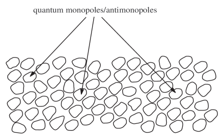
Figure 3: QCD vacuum $\approx$ stochastic gas of quantum monopoles/antimonopoles.

VIII Acknowledgment

VD is grateful for Viktor Gurovich for the fruitful discussion, ISTC grant KR-814 for the financial support and Alexander von Humboldt Foundation for the support of this work.

References

- (1) P.A.M. Dirac, Proc. Roy. Soc., A133, 60 (1931); P.A.M. Dirac, Phys. Rev. 74, 817 (1949)
- (2) G. ’t Hooft, Nucl. Phys. B79, 276 (1974); A.M. Polyakov, JETP Lett. 20, 194 (1974)
- (3) M. I. Polikarpov, “Recent results on the Abelian projection of lattice gluodynamics,” Nucl. Phys. Proc. Suppl. 53, 134 (1997), hep-lat/9609020.
- (4) W. Heisenberg, Nachr. Akad. Wiss. Göttingen, N8, 111 (1953); W. Heisenberg, Nachr. Akad. Wiss. Göttingen; W. Heisenberg, Zs. Naturforsch., 9a, 292 (1954); W. Heisenberg, F. Kortel and H. Mütter, Zs. Naturforsch., 10a, 425 (1955); W. Heisenberg, Zs. für Phys., 144, 1 (1956); P. Askali and W. Heisenberg, Zs. Naturforsc., 12a, 177 (1957); W. Heisenberg, Nucl. Phys., 4, 532 (1957); W. Heisenberg, Rev. Mod. Phys., 29, 269 (1957)
- (5) W. Heisenberg, Introduction to the Unified Field Theory of Elementary Particles., Max-Planck-Institute für Physik und Astrophysik, Interscience Publishers London, New York, Sydney, 1966
- (6) T.T. Wu and C.N. Yang Properties of Matter Under Unusual Conditions, ed. H. Mark and S. Fernbach (Interscience, New York 1968)
- (7) E. Eichten, et. al., Phys. Rev. D17, 3090 (1978)
- (8) D. Singleton and A. Yoshida, Int. J. Mod. Phys. A12, 4823 (1997)
- (9) G. t’Hooft, Nucl. Phys., B190, 455 (1981); Proccedings of the Workshop “Confinement, Duality and Non-perturbative Aspects of QCD”, Cambridge (UK), 24 June - 2 July, 1997.
- (10) A.S. Kronfeld, M.L. Laursen and U.J. Wiese, Phys. Lett. 190B, 516(1987); A.S. Kronfeld, G. Schierholz and U.J. Wiese, Nucl. Phys. B293, 461 (1987).
- (11) T. Shinohara, T. Imai and K. I. Kondo, “The most general and renormalizable maximal Abelian gauge,”, hep-th/0105268.
- (12) M. N. Chernodub and M. I. Polikarpov, “Abelian projections and monopoles,”, hep-th/9710205.
- (13) V. Dzhunushaliev, Phys. Rev, B64, 024522 (2001).
- (14) V. Dzhunushaliev and D. Singleton, Int. J. Theor. Phys, 38, 887(1999); hep-th/9912194.
- (15) V. Dzhunushaliev, Phys. Lett. B498, 218 (2001); hep-th/0010185
- (16) C.G. Callan, R. Dashen and D.J. Gross, Phys. Lett. B66, 375 (1977); Phys Rev. D17, 2717 (1978); Phys. Rev. D19, 1826 (1979)
- (17) J.V. Steele and J.W. Negele, Phys. Rev. Lett., 85, 4207 (2000)
- (18) J.W. Negele, “Instanton and Meron Physics in Lattice QCD”, hep-lat/0007027; J.V. Steele, “Can Merons Describe Confinement?”, hep-lat/0007030
- (19) G. t’Hooft, in Proc. Europ. Phys. Soc. Conf. on High Energy Physics (1975), p.1225.
- (20) S. Mandelstam, Phys. Rev. D19, 2391 (1979).
- (21) T. Suzuki and I. Yotsuyanagi, Phys. Rev. D42, 4257(1990); J.D. Stack, S.D. Neiman and R.J. Wensley, Phys. Rev. D50, 3399(1994); M.N. Chernodub and M.I. Polikarpov, “Abelian projections and monopoles”, hep-th/9710205.