Density Matrix Renormalization Group Approach to the Massive Schwinger Model

Abstract

The massive Schwinger model is studied, using a density matrix renormalization group approach to the staggered lattice Hamiltonian version of the model. Lattice sizes up to 256 sites are calculated, and the estimates in the continuum limit are almost two orders of magnitude more accurate than previous calculations. Coleman’s picture of ‘half-asymptotic’ particles at background field $\theta=\pi$ is confirmed. The predicted phase transition at finite fermion mass $(m/g)$ is accurately located, and demonstrated to belong in the 2D Ising universality class.

The Schwinger model[1], or quantum electrodynamics in one space and one time dimension, exhibits many analogies with QCD, including confinement, chiral symmetry breaking, charge shielding, and a topological $\theta$-vacuum[2, 3, 4]. It is a common test bed for the trial of new techniques for the study of QCD: for instance, several authors have discussed new methods of treating lattice fermions using the Schwinger model as an example [5].

Our purpose in this paper is twofold. First, we aim to explore the physics of this model when an external ‘background’ electric field is applied, as discussed long ago in a beautiful paper by Coleman[4]. Secondly, we wish to demonstrate the application of density matrix renormalization group (DMRG) methods [6, 7] to a model of this sort, with long-range, non-local Coulomb interactions. The DMRG approach has been used with great success for lattice spin models and lattice electron models such as the Hubbard model; here we apply it to a lattice gauge model.

Choosing a time-like axial gauge $A_{0}=0$, the Schwinger model Hamiltonian becomes

$$H=\int dx\left(-i\bar{\psi}\gamma^{1}(\partial_{1}+igA_{1})\psi+m\bar{\psi}\psi+\frac{1}{2}E^{2}\right).$$ (1)

where $\psi$ is a 2-component spinor field, since there is no spin in one space dimension. The coupling $g$ has dimensions of mass, so the theory is super-renormalizable. Using $g$ as the scale of energy, the physical properties of the model are then functions of the dimensionless ratio $m/g$. Gauss’ law becomes

$$\partial_{1}E=-\partial_{1}\dot{A}^{1}=gj^{0}=g\bar{\psi}\gamma^{0}\psi.$$ (2)

where $E$ is the 1-component electric field. This can be integrated to give

$$E=g\int dxj^{0}(x)+F,$$ (3)

showing that $E$ is not an independent field, but can be determined in terms of the charge density $j^{0}(x)$, up to the constant of integration $F$, which corresponds to a “background field”, as discussed by Coleman [4]. We can think of the background field as created by condenser plates at either end of our one-dimensional universe.

If $|F|>g/2$, charged pairs will be produced, and separate to infinity, until the field is reduced within the range $|F|\leq g/2$, thus lowering the electrostatic energy per unit length. Thus physics is periodic in $F$ with period $g$, and it is convenient to define an angle $\theta$ by $\theta=2\pi F/g$. Then we can always choose $\theta$ to lie in the interval $[0,2\pi]$.

In the weak-coupling limit $m/g\rightarrow\infty$, the vacuum contains no fermionic excitations, and the vacuum energy density $\epsilon_{0}$ is given purely by the electrostatic energy term (we ignore the energy of the Dirac sea) $\epsilon_{0}=F^{2}/2$ $(\theta\leq\pi)$ or $(g-F)^{2}/2$ $(\pi\leq\theta\leq 2\pi)$.

Thus there is a discontinuity in the slope of the energy density, corresponding to a first-order phase transition, at $\theta=\pi$. In the strong-coupling limit $m/g=0$, on the other hand, chiral invariance demands that the vacuum energy density remains constant as a function of $\theta$[4]. Thus we expect a first-order transition at $\theta=\pi$ for large $m/g$, which terminates at a second order critical point at some finite $(m/g)_{c}$. The two-fold vacuum degeneracy would naturally lead one to expect that the transition will lie in the Ising universality class.

Normally, charge is confined in the model: there is a ‘string’ of constant electric field (or flux) connecting any pair of opposite charges [2, 3]. But Coleman [4] points out that in the very special case $\theta=\pi$, the peculiar phenomenon of “half-asymptotic” particles arises. In the weak-coupling limit, one can envisage the state shown in Fig. 1. The electric field energy density is the same in between each pair of particles, and they can therefore move freely, as long as they maintain the same ordering, i.e. no pair of fermions interchanges positions.

The one-dimensional fermionic theory can be mapped into an equivalent Bose form [3, 8]. At $m/g=0$, the theory is exactly solvable, and reduces to a theory of free, massive bosons, with mass $M=g/\sqrt{\pi}$, independent of the background field $\theta$. At large $m/g$ and $\theta=\pi$, where the spontaneous symmetry breaking occurs, the half-asymptotic particles are found to correspond to topological solitons, or “kinks” and “antikinks”, in the Bose language [4].

There have been very few attempts to verify these predictions numerically, that we are aware of. Hamer, Kogut, Crewther and Mazzolini[9] used finite-lattice techniques to address the problem, and located the phase transition at $\theta=\pi$ to lie at $(m/g)_{c}=0.325(20)$, with a correlation length index $\nu=0.9(1)$. Schiller and Ranft [11] used Monte Carlo techniques to locate the phase transition at $(m/g)_{c}=0.31(1)$. For zero background field, on the other hand, many different numerical methods have been applied to the Schwinger model; for a recent review, see Sriganesh et al. [10].

We employ the Kogut-Susskind [12] Hamiltonian lattice formulation of the Schwinger model, following Banks et al. [13]. The dimensionless lattice Hamiltonian is

$$W=\frac{2}{ag^{2}}H=\sum_{n}L^{2}(n)+\mu\sum_{n}(-1)^{n}\phi^{\dagger}(n)\phi(n)-ix\sum_{n}\left[\phi^{\dagger}(n)e^{i\theta(n)}\phi(n+1)-\mbox{h.c.}\right]$$ (4)

where $a$ is the lattice spacing, $\phi(n)$ is a single-component fermion field at site $n$, $e^{i\theta(n)}$ is the link variable at link $n$, and $\mu=2m/(g^{2}a)$, $x=1/(g^{2}a^{2})$.

We use a “compact” formulation where the gauge field becomes an angular variable $0\leq\theta(n)\leq 2\pi$ on the lattice, and $L(n)$ is the conjugate spin variable (the lattice equivalent of the electric field)

$$[\theta(n),L(m)]=i\delta_{nm}$$ (5)

so that $L(n)$ has integer eigenvalues $L(n)=0,\pm 1,\pm 2,\dots$.

In the lattice strong-coupling limit $x\rightarrow 0$, the unperturbed ground state $|0\rangle$ has

$$L(n)=0,\ \ \ \ \ \phi^{\dagger}(n)\phi(n)=\frac{1}{2}[1-(-1)^{n}],\ \ \ \ \ \mbox{all }n$$ (6)

whose energy we normalize to zero. The lattice version of Gauss’ law is then taken as

$$L(n)-L(n-1)=\phi^{\dagger}(n)\phi(n)-\frac{1}{2}[1-(-1)^{n}]$$ (7)

which means excitations on odd and even sites create $\mp 1$ units of flux, corresponding to “electron” and “positron” excitations respectively. Eq. (7) determines the electric field $L(n)$ entirely, up to an arbitrary additive constant $\alpha$, which then represents the background field. Allowing $\alpha$ to be non-zero, the electrostatic energy term is modified to $\sum_{n}L^{2}(n)\rightarrow\sum_{n}(L(n)+\alpha)^{2}$. The physics of the background field then matches precisely with the continuum discussion. Physics is then periodic in $\alpha$ with period 1, and the background field variable is $\theta=2\pi\alpha$ .

In the weak-coupling limit $m/g\rightarrow\infty$ and for background field $\alpha=1/2$, there are two degenerate vacuum or ‘loop’ states, $|\frac{1}{2}\rangle$ and $|-\frac{1}{2}\rangle$, corresponding to $\{L(n)+\alpha=\pm 1/2,\mbox{ all }n\}$, respectively. On a finite lattice, the eigenstates will be the symmetric and anti-symmetric combinations of those, and we will denote the energy gap between them by $\Delta_{0}$. The single-fermion state will consist of a single electron with $L(n)+\alpha=+1/2$ to its left and $-1/2$ to its right; the energy gap between this and the ground state will be denoted $\Delta_{1}$. Finally, the energy gap to the lowest 2-particle electron-positron state will be denoted $\Delta_{2}$.

We will also study two order parameters which can be used to characterize the phase transition at $\theta=\pi$. The first one is the average electric field

$$\Gamma^{\alpha}=\frac{1}{N}\langle\sum_{n}(L(n)+\alpha)\rangle_{0},$$ (8)

which in the weak-coupling limit $m/g\rightarrow\infty$ takes values $\pm 1/2$ for the zero-loop and one-loop states respectively. The second order parameter is the axial fermion density suggested by Creutz[5]

$$\Gamma^{5} = \langle i\bar{\psi}\gamma^{5}\psi/g\rangle_{0}$$ (9)

$$= -\frac{i\sqrt{x}}{N}\langle\sum_{n}(-1)^{n}\left[\phi^{\dagger}(n)\phi(n+1)-\mbox{h.c.}\right]\rangle_{0}.$$ (10)

Our results are based on the density matrix renormalization group (DMRG) method [6, 7]. The method employed here is the “infinite system” DMRG method, as prescribed by White [6], used both with open and periodic boundary conditions (OBC and PBC). Due to the presence of the electric field on the links, and the differing nature of the odd and even-numbered sites, some modifications were made to the method, although nothing that changes the spirit of the DMRG.

For a particular spin configuration with OBC, if we specify the incoming electric field for the first site of the chain, then according to Gauss’s law the electric field for all the links can be deduced. If PBC are imposed, then as there is no particular link to fix the electric field, we can have loops of electric flux extending throughout the ring. In the presence of a background field we simply add (or subtract) $\alpha$ from the values of the electric fields due to the spin configuration. A cutoff, or maximum loop value was chosen such that full convergence was reached to machine precision. A loop range of [-5,5] was more than sufficient in most cases.

In the standard “infinite system” method one splits the chain (or ring) into two blocks and two sites, and in each DMRG iteration the blocks increase in size by a single site. Due to the differing nature of the odd and even sites in the lattice formulation (4), we modify this so that two sites are augmented each time, so that the superblock grows by four sites in a single DMRG iteration. We truncate the basis in each DMRG iteration such that there are a maximum of 125 states per spin sector per loop in a block.

The accuracy of the DMRG calculation is strongly dependent on the parameter values $x$ and $m/g$. In the worst case scenario $(m/g=0.3;x=100;\theta=\pi;N=256)$ with PBC, which represents the smallest lattice spacing used for this study, and lies in the critical region, the ground state energy can be resolved to 1 part in $10^{6}$, while the two-particle gap is resolved to 1 part in $10^{3}$, while the order parameters are accurate to 3 figures. It is more usual to obtain ground state eigenvalues to near machine precision, and “vector” gap errors of 1 part in $10^{6}$.

We begin with the case of zero background field, $\theta=0$, in order to demonstrate the power of the DMRG method. The most accurate results to date are those of Sriganesh et al. [10], who used exact diagonalization on lattices up to $N=22$ sites. With DMRG it is possible to go to $N=256$ sites, such that there is essentially no extrapolation necessary to obtain the bulk limit $N\rightarrow\infty$. Fig. 2 shows the data for $m/g=0$, which is the exactly soluble case. For $x=4$ through to $x=100$ we have 6 figure convergence. The final continuum limit $a\rightarrow 0$ or $x\rightarrow\infty$ is obtained by making polynomial fits in powers of $1/\sqrt{x}=ga$ as used in Ref. [10]. Our final estimate of $m^{-}/g=0.56419(4)$ for this case agrees extremely well with the analytic result of $1/\sqrt{\pi}=0.5641896..$, and is about 25 times more accurate than the corresponding estimate $0.563(1)$ by Sriganesh et al. [10].

We now turn to the case of background field $\theta=\pi$. First, we use finite-size scaling theory to estimate the position of the critical point, by calculating “pseudo-critical points” at each lattice size $N$, and each lattice spacing $x$. The pseudo-critical point is defined[15] as the point where two successive finite-lattice energy gaps scale like $1/N$. For this exercise we used the ‘loop gap’ $\Delta_{0}/g$, which collapses to zero at the pseudo-critical point. The pseudo-critical points converge very rapidly to the bulk limit, like $1/N^{3}$. The results are shown in Fig. 3. A quadratic fit in $1/\sqrt{x}$ extracts the continuum limit, which we estimate to be $(m/g)_{c}=0.3335(2)$. This is consistent with the previous estimates by Hamer et al. [9] of $(m/g)_{c}=0.325(20)$, or Schiller and Ranft [11], $(m/g)_{c}=0.31(1)$, but with two orders of magnitude improvement in accuracy.

Finite-size scaling theory [15] also allows us to estimate the critical indices for the model. The order parameters $\Gamma^{\alpha}_{N}$ and $\Gamma^{5}_{N}$, for instance, are expected to scale like $\sim N^{-\beta/\nu}$ [15]. Then the logarithmic ratios

$$\frac{\ln[\Gamma_{N}((m/g)_{N}^{*})/\Gamma_{N-1}((m/g)_{N}^{*})]}{\ln[N/(N-1)]}\sim-\frac{\beta}{\nu}$$ (11)

give a direct estimate of the index ratio. Fig. 4 shows the resulting estimates for $\beta/\nu$, obtained from the electric field order parameter, and for $1/\nu$, obtained from the beta function. We see essentially no variation in the exponents with lattice spacing, to within the accuracy of our calculations. Our best estimates for the critical exponents are thus $\nu=0.99(1)$, $\beta/\nu=0.125(5)$. These results provide reasonably conclusive evidence that the Schwinger model transition at $\theta=\pi$ lies in the same universality class as the one dimensional transverse Ising model, or equivalently the 2D Ising model, with ($\nu=1,\beta=1/8$).

We now turn to estimating continuum limit values for the energy gaps and order parameters. The convergence at $\theta=\pi$ is not so good as at $\theta=0$. Fig. 5 displays our final results for the energy gaps $\Delta_{0}/g$ between the “loop” states, $\Delta_{1}/g$ in the 1-particle sector, and $\Delta_{2}/g$ in the 2-particle sector, for all values of $m/g$.

We see that all gaps vanish at the critical point. The ‘loop’ gap is zero for all $m/g>(m/g)_{c}$, as predicted by Coleman [4]. The 2-particle gap $\Delta_{2}/g$ vanishes at the critical point $(m/g)_{c}$, but on either side of the critical point there is a finite gap, and an almost linear behavior with $m/g$. Note, however, that the behavior is not exactly linear. The 1-particle gap vanishes for $m/g<(m/g)_{c}$, while for $m/g>(m/g)_{c}$ it is very close to half the 2-particle gap. Once again, the behavior is very nearly linear in $m/g$.

The pattern of eigenvalues exhibited in Fig. 5 bears an extraordinary resemblance to that of the transverse Ising model [16]. In particular, we see that the energy of the 1-particle or ‘kink’ state vanishes at the critical point, and then remains degenerate with the ground state for $(m/g)<(m/g)_{c}$. Assuming this degeneracy is exact, this indicates that a ‘kink condensate’ will form in the ground state for small mass, as discussed by Fradkin and Susskind[16]. It also indicates the existence of a new ‘dual symmetry’ in the model, which is spontaneously broken in the low-mass region, and has not been explored hitherto. There should also be a ‘dual order parameter’ associated with this symmetry.

We may also obtain estimates for the order parameters $\Gamma^{5}$ and $\Gamma^{\alpha}$ as functions of $m/g$. Our results are displayed in Fig. 6. Both order parameters are zero, within errors, for $m/g<(m/g)_{c}$. It appears that both order parameters turn over and drop abruptly to zero as the critical point is approached from above, consistent with the small exponent $\nu=1/8$ found previously. The axial density $\Gamma^{5}$ decreases steadily towards zero at large $m/g$, whereas $\Gamma^{\alpha}$ approaches the expected value of $1/2$. More detailed results will be given in a forthcoming paper[14].

We would like to thank Profs. Michael Creutz and Jaan Oitmaa and Dr. Zheng Weihong for useful discussions and help. We are grateful for computational facilities provided by The New South Wales Center for Parallel Computing, The Australian Center for Advanced Computing and Communications and The Australian Partnership for Advanced Computing. R.B. was supported by The Australian Research Council and The J. G. Russell Foundation.

FIG. 1.: A configuration of “half-asymptotic” charged fermions at background field $F=g/2$.

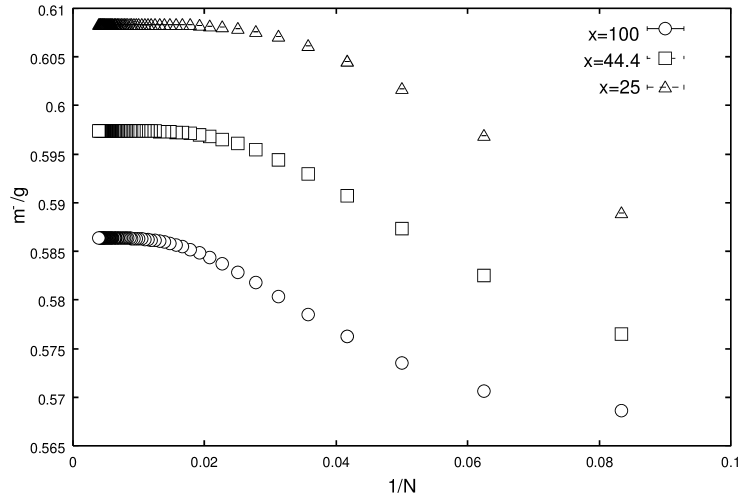
FIG. 2.: “Vector” mass gaps for $m/g=0$, finite lattices $N=10$-$256$, and various lattice spacings.

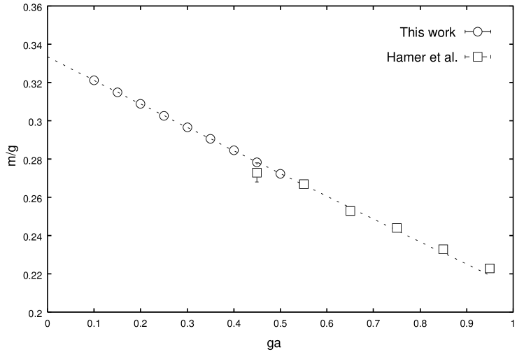
FIG. 3.: Critical line in the $m/g$ versus $1/\sqrt{x}=ga$ plane. Open circles are our present estimates, and squares are the previous results of Hamer et al. [9], which are in good agreement. The dashed line is a quadratic fit to the data in $ga$.

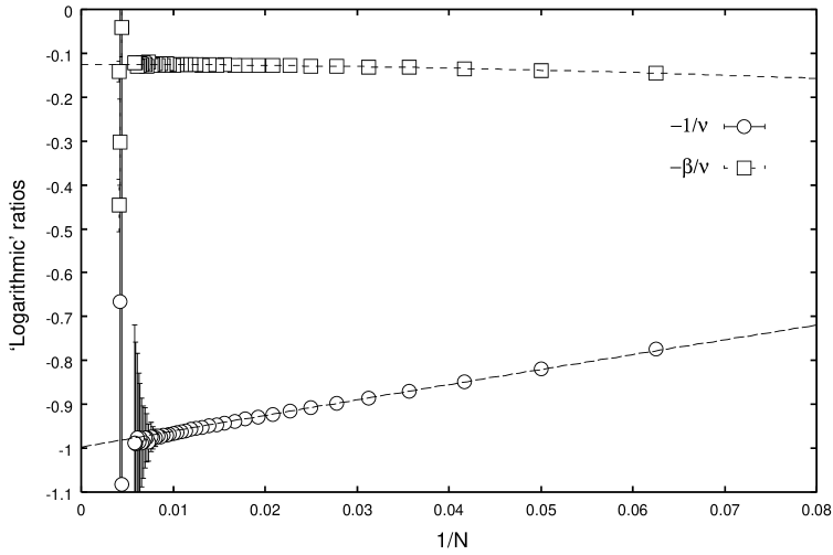
FIG. 4.: ‘Logarithmic’ ratio estimates of critical indices $-1/\nu$ and $-\beta/\nu$ for lattice spacing $1/\sqrt{x}=ga=0.45$. Quadratic fits in $1/N$ provide the bulk extrapolations. We estimate here $1/\nu=1.00(2)$ and $\beta/\nu=0.125(5)$.

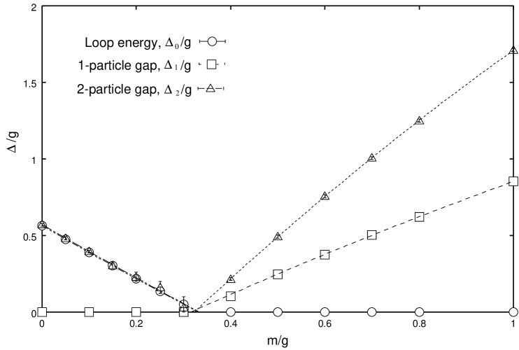
FIG. 5.: Final estimates for gaps in the 0-particle, 1-particle and 2-particle sectors at $\theta=\pi$. Dashed lines are merely to guide the eye.

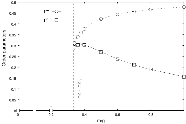
FIG. 6.: Order parameters $\Gamma^{\alpha}=\langle(L+\alpha)\rangle_{0}$ , $\Gamma^{5}=\langle i\bar{\psi}\gamma_{5}\psi/g\rangle_{0}$ near the critical region. Dashed lines are merely to guide the eye.

REFERENCES

- [1] J. Schwinger, Phys. Rev. 128, 2425 (1962).
- [2] A. Casher, J. Kogut, and L. Susskind, Phys. Rev. D 10, 732 (1974).
- [3] S. Coleman, R. Jackiw, and L. Susskind, Ann. of Phys. 93, 267 (1975).
- [4] S. Coleman, Ann. of Phys. 101, 239 (1976).
- [5] M. Creutz, Nucl. Phys. Proc. Suppl. 42, 56 (1995).
- [6] S.R. White, Phys. Rev. Lett. 69, 2863 (1992); Phys. Rev. B 48, 10345 (1993).
- [7] G.A. Gehring, R.J. Bursill and T. Xiang, Acta Phys. Pol. 91, 105 (1997).
- [8] S. Mandelstam, Phys. Rev. D 11, 3026 (1975).
- [9] C.J. Hamer, J. Kogut, D.P. Crewther, and M.M. Mazzolini, Nucl. Phys. B208, 413 (1982).
- [10] P. Sriganesh, C.J. Hamer and R.J. Bursill, Phys. Rev. D 62, 034508 (2000).
- [11] A.J. Schiller and J. Ranft, Nucl. Phys. B225, 204 (1983).
- [12] J. Kogut and L. Susskind, Phys. Rev. D 11, 395 (1975).
- [13] T. Banks, L. Susskind, and J. Kogut, Phys. Rev. D 13, 1043 (1976).
- [14] T. Byrnes et al., in preparation.
- [15] M.N. Barber, in Phase Transitions and Critical Phenomena, vol. 8, edited by C. Domb and J. Lebowitz (Academic, New York, 1983).
- [16] E. Fradkin and L. Susskind, Phys. Rev. D17, 2637 (1978).