MIT-CTP-3217

ON THE NON-PERTURBATIVE GLUON MASS
AND HEAVY QUARK PHYSICS

Owe Philipsen

Center for Theoretical Physics,
Massachusetts Institute of Technology,
Cambridge, MA 02139-4307, USA

We study a recently proposed gauge invariant, non-local pure gauge observable, which is equivalent to the gluon propagator in a certain gauge. The correlator describes a gluon coupled to static sources and decays with eigenvalues of the Hamiltonian, permitting a non-perturbative definition of a gluonic parton mass. Detailed numerical tests of the observable are performed in SU(2) gauge theories in 2+1 dimensions. In a Higgs model it reproduces the physical W-boson mass, while in a confining theory its non-local nature results in almost exclusive projection onto torelonic states. However, the gluon mass can also be related to the mass difference between the lowest gluelumps, i.e. gluon configurations bound to adjoint sources. Its value is computed in SU(2) pure gauge theory in 2+1 dimensions to be $m_{A}=0.360(19)g^{2}$, which plays an important role as “magnetic mass” of the four-dimensional theory at high temperatures. The same quantity is found to determine the mass splitting between vector and scalar mesons in the three-dimensional theory. In SU(3) pure gauge theory in 3+1 dimensions the corresponding gluelump splitting yields $m_{A}\approx 370$ MeV. Possible relations of this quantity with the QCD heavy meson spectrum are discussed.

1 Introduction

The physics of confinement of quarks in QCD is well established experimentally and by numerical simulations of lattice gauge theories. However, little is known about the confiment mechanism, i.e. how parton physics at short distances smoothly evolves into hadron physics at large distances. Understanding this transition requires non-perturbative knowledge of the parton dynamics at all length scales. Such knowledge is indispensable in the context of finite temperature and baryon density, where matter is believed to appear in a deconfined state whose collective physical properties are determined by parton dynamics. The latter is encoded in the Green functions of quark and gluon fields, which in general are not gauge invariant. This raises the conceptual problem of how to define non-perturbative partons and extract physical information about them. In this work an attempt is made to answer this question for a suitably defined gluon correlation function. Once this most elementary case is understood, it may be generalized to quarks and more complex Green functions.

In perturbation theory one fixes a gauge and studies partons directly. Although field propagators are gauge dependent and not physical observables, they carry gauge invariant information about the parton dynamics in their singularity structure. Pole masses defined from the gluon and quark propagators have been proved to be gauge independent to every finite order in perturbation theory [1, 2]. However, perturbation theory is limited by the requirement of weak coupling. On the other hand, numerical results obtained by fixing a gauge on the lattice [3] have often been inconclusive or controversial in the past. This is due to the difficulty to fix a gauge uniquely and avoid the problem of Gribov copies [4]. Moreover, most complete gauge fixings (e.g. the Landau gauge) violate the positivity of the transfer matrix, thus obstructing a quantum mechanical interpretation of the results. Finally, gauge independence of any result is not evident, but has to be demonstrated numerically by comparing different gauges, while it is extremely difficult to control the mentioned problems for each gauge. An overview with references to numerical work may be found in [5].

A non-perturbative argument for a non-zero dynamical mass scale associated with gluons was given a long time ago [6], based on the static potential of adjoint sources. If gluons were non-perturbatively massless, they could be pair produced at no energy cost and the adjoint potential would be screened even for small separations. In lattice simulations, by contrast, one observes a linear rise up to rather large distances, until the adjoint string breaks at $\sim 10M_{G}^{-1}$, in units of the lightest glueball [7, 8].

Recently, non-local, gauge invariant observables have been constructed in lattice gauge theory which are equivalent to the gluon propagator in certain gauges. The transfer matrix formalism has been used to prove that these gluon correlators decay exponentially with eigenvalues of the Hamiltonian [9], implying a pole structure in momentum space. The energy gap between the vacuum and the lowest excited eigenvalue then represents a gauge invariant definition for a gluonic parton mass.

The purpose of the current work is to compute the value of the gluon mass in pure gauge theory and to establish its relation to physical observables. The main results are as follows: A gauge invariant probe of the gluon energy is obtained by coupling it to external static sources and measuring the energy of the composite object. The problem is then reduced to separate the contribution of the gluon field from that of the sources. In principle, this can be achieved in two ways. First, by dressing the field variables with a non-local functional representing an average over all positions of the sources. Second, by introducing explicit fields for the sources, which can be integrated over analytically. In both cases the resulting gauge invariant observables can be related to the gluon propagator in a particular gauge. The second procedure has the advantage of being local and numerically feasible in a confining theory. Moreover, it lends itself to a straightforward interpretation of the gluon mass, whose value equals that of the level splitting between the lightest “gluelumps”, i.e. gluonic configurations coupled to an adjoint source. The latter can be computed straightforwardly without need for gauge fixing or introduction of non-local fields. We calculate its value for SU(2) Yang-Mills theory in 2+1 dimensions and find $m_{A}=0.36(2)g^{2}$. This result plays an important role for the four-dimensional high temperature physics, where it corresponds to the magnetic mass with $g^{2}\sim g_{4d}^{2}T$. For SU(3) in 3+1 dimensions, the same splitting has been computed in the literature to be $m_{A}=368(7)$ MeV [10]. In three dimensions one furthermore finds the splitting of heavy vector and scalar mesons to be given by the gluon mass. The situation in QCD might be similar, but a careful study of the static limit is necessary to settle this question.

The outline of the paper is as follows. In Sec. 2 we review the Hamiltonian formalism of lattice gauge theory, which in its strong coupling limit permits a natural definition of a gauge invariant mass gap in terms of a gluon coupled to external sources. Sec. 3 recalls the main results of [9], relating the Hilbert space definition to a non-local Euclidean observable amenable to numerical simulations. This operator is tested in 2+1 dimensional theories in Sec. 4. The relation to the gluelump spectrum is derived in Sec. 5, and numerical results are quoted for SU(2) in 2+1 and SU(3) in 3+1 dimensions. Finally, Sec. 6 discusses the connection to the heavy meson spectrum for SU(2) in 2+1 dimensions as well as QCD, before conclusions are given in Sec. 7. A continuum formulation of gluons probed by sources as well as lattice actions and parameters used in the simulations are given in two appendices.

2 The gluon in the Hamiltonian formalism

To begin, it is instructive to recall the Hamiltonian formulation of lattice gauge theory [11], where it is easy to see that gauge invariant information is associated with field variables and how it can be interpreted physically. We are interested in SU(N) gauge theory on an $L^{d}\times N_{t}$ lattice with periodic boundary conditions. In a Hilbert space formulation [11, 12, 13] a spatial sublattice $L^{d}$ at a fixed time is considered, with link variables $U_{i}({\bf x})$ and the corresponding field operators $\hat{U}_{i}({\bf x})$. The wave functions form a Hilbert space ${\cal{H}}_{0}$ of all complex, square integrable functions $\psi[U]$ defined on the gauge group $G$: ${\cal{H}}_{0}=[L^{2}(G)]^{dL^{d}}$. A unitary operator $\hat{R}(g)$ imposes gauge transformations $g({\bf x})\in G$ on wave funtions according to

$$\left(\hat{R}\psi\right)[U]=\psi[U^{g}],\qquad U_{i}^{g}({\bf x})=g({\bf x})U_{i}({\bf x})g^{{\dagger}}({\bf x}+\hat{\i})\,.$$ (2.1)

Wave functions of physical particle states are gauge invariant, $\psi[U^{g}]=\psi[U]$, thus forming a subspace $\cal{H}\subset$${\cal H}_{0}$. Any wave function $\psi[U]\in{\cal{H}}_{0}$ can be projected on the physical subspace by means of the projection operator $\hat{P}$,

$$(\hat{P}\psi)[U]=\int\prod_{{\bf x}}dg({\bf x})\;\psi[U^{g}].$$ (2.2)

The Kogut-Susskind Hamiltonian acting on the full space ${\cal H}_{0}$ is obtained by quantizing the theory in temporal gauge $U_{0}=1$ and reads [11]

$$\hat{H}_{0}=\frac{g^{2}}{2a^{d-2}}\sum_{{\bf x},i}(\hat{E}_{i}^{a}({\bf x}))^{2}-\frac{2}{g^{2}a^{4-d}}\sum_{{\bf x},i<j}\mathop{\rm Re}{\rm Tr\,}\hat{P}_{ij}({\bf x})\,,$$ (2.3)

where $P_{ij}({\bf x})=U_{i}({\bf x})U_{j}({\bf x}+\hat{\i})U_{i}^{\dagger}({\bf x}+\hat{\i}+\hat{\j})U_{j}^{\dagger}({\bf x})$ is the elementary plaquette field. The components of electric field and link operators satisfy the commutation relations

$$\left[\hat{E}_{i}^{a}({\bf x}),\hat{E}_{j}^{b}({\bf y})\right] = {\rm i}f_{abc}\hat{E}_{i}^{c}({\bf x})\delta_{ij}\delta_{{\bf x}{\bf y}},$$

$$\left[\hat{E}_{i}^{a}({\bf x}),\hat{U}_{j,\alpha\beta}({\bf y})\right] = -T^{a}\hat{U}_{i,\alpha\beta}({\bf x})\delta_{ij}\delta_{{\bf x}{\bf y}}.$$ (2.4)

In principle the whole configuration space may be constructed by applying link operators in all possible combinations to the vacuum state, $\psi_{0}=1$. In particular, doing this just once we have

$$\psi^{1}_{\alpha\beta}[U]\equiv{\hat{U}}_{i,\alpha\beta}({\bf x})\psi_{0}=U_{i,\alpha\beta}({\bf x})\psi_{0}.$$ (2.5)

Thus, $\psi^{1}[U]$ is the wave function corresponding to one link variable being excited and all others being in the vacuum configuration. Clearly, it transforms non-trivially, $\psi^{1}_{\alpha\beta}[U^{g}]=g_{\alpha\gamma}({\bf x})g^{*}_{\beta\delta}({\bf x}+\hat{\i})\psi_{\gamma\delta}[U]$. Gauge invariant wave functions are obtained by exciting closed loops of links, the simplest being a plaquette, $\psi^{P}[U]=P_{ij}({\bf x})$.

In the limit of strong coupling, $a^{(3-d)}g^{2}\rightarrow\infty$, the potential term in the Hamiltonian decouples. Although this limit is far from the continuum and the physical situation, it illustrates the structure of the Hilbert space ${\cal H}_{0}$. In the strong coupling limit $\psi^{1}$ is an eigenstate of the Hamiltonian,

$$\hat{H}_{0}\psi_{\alpha\beta}^{1}[U]=E_{1}\psi_{\alpha\beta}^{1}[U],\quad E_{1}=\frac{g^{2}}{2a^{d-2}}C_{F},\quad C_{F}=(N^{2}-1)/2N.$$ (2.6)

Excitation of other links increases the energy by one unit for every link. The wave function for a string of electric flux between charges at ${\bf x},{\bf y}={\bf x}+l\hat{\i}$,

$$\psi^{S}_{\alpha\beta}[U]=[U_{i}({\bf x})U_{i}({\bf x}+\hat{\i})\ldots U_{i}({\bf x}+(l-1)\hat{\i})]_{\alpha\beta}=U_{\alpha\beta}({\bf x},{\bf y}),$$ (2.7)

is an eigenstate with energy $lE_{1}$, whereas $\psi^{P}[U]$ has energy $4E_{1}$. The plaquette wave function is in the Hilbert space of gauge invariant functions, $\psi^{P}[U]\in\cal{H}$. On the other hand, the wave functions $\psi^{1,S}$ are non-invariant and hence not elements of the projected Hilbert space. Nevertheless, because time independent gauge transformations commute with the Hamiltonian, $[\hat{R},\hat{H}]=0$, the eigenvalues belonging to these wave functions are gauge invariant.

It is now natural to define a “gluon mass gap” by the energy it takes to excite one gluon configuration out of the vacuum. Defining the usual lattice gluon field

$$A_{i}({\bf x})=\frac{{\rm i}}{2g}\left[U_{i}({\bf x})-U^{{\dagger}}_{i}({\bf x})-\frac{1}{N}{\rm Tr\,}\left(U_{i}({\bf x})-U^{{\dagger}}_{i}({\bf x})\right)\right],$$ (2.8)

one has for the corresponding wave function $\psi^{A}_{\alpha\beta}[U]=\hat{A}_{i,\alpha\beta}({\bf x})\psi_{0}$ in the strong coupling limit

$$\hat{H}_{0}\psi^{A}_{\alpha\beta}[U]=E_{1}\psi^{A}_{\alpha\beta}[U].$$ (2.9)

Hence, in the Hamiltonian strong coupling limit the gluon has a gauge invariant mass gap, which is an eigenvalue of $\hat{H}_{0}$ to a gauge covariant eigenfunction. Note that the wave functions for a unit of flux and the gluon wave function are constructed from the same link variable. The difference is in the transformation property. $\psi^{A}$ picks the traceless part of the link variable only, and hence is an ($N^{2}-1$)-plet of the form $\sim c^{a}[U]T^{a}$ with some real functions $c^{a}[U]$.

Away from the strong coupling limit the energy levels and the precise form of the eigenstates will change. However, their transformation properties remain the same since gauge transformations commute with the full Hamiltonian. Quite generally, eigenstates with non-trivial transformation behaviour describe strings of flux with energy $E$. They can be made manifestly gauge invariant and “physical” by letting the flux end on static sources. The total wave functions then are gauge invariant combinations of the wave function for the source, $\phi^{g}({\bf x})=g({\bf x})\phi({\bf x})$, and the gauge part,

$$\psi^{1,S}_{tot}[U]=\phi^{*}_{\alpha}({\bf x})\phi_{\beta}({\bf x}+\hat{\i})\psi^{1,S}_{\alpha\beta}[U],\quad\psi^{A}_{tot}[U]=\frac{{\rm i}}{2g}\left(\psi^{1}_{tot}[U]-\psi^{1{\dagger}}_{tot}[U]\right).$$ (2.10)

In summary, in addition to the gauge invariant particle states of $\cal{H}$, ${\cal H}_{0}$ contains additional states describing static potentials, or gauge field configurations probed by external charges. The corresponding pure gauge wave functions transform non-trivially, but the associated energies are fully gauge invariant and contain valuable information about the dynamics of charged states. In this respect a gluon wave function is on the same footing as a wave function for a flux element, whose traceless part it constitutes. We conclude that a gluon mass may be defined by the minimal energy it takes to excite a flux element in an $(N^{2}-1)$ or adjoint state. This energy is not related to an asymptotic particle state, but rather a field coupled to static sources. The expression Eq. (2.10) suggests that it is a short distance property of the static potential with the sources and the flux in an adjoint state.

2.1 Transfer matrix and Euclidean correlation functions

In order to make the spectrum amenable to numerical simulations, the Hilbert space picture has to be connected to Euclidean correlation functions by means of the transfer matrix [12, 13]. The latter is an integral operator translating the wave functions in time,

$$\psi[U_{t+1}] = \left(\hat{T}_{0}\psi\right)[U_{t}]$$ (2.11)

$$= \int\prod_{{\bf x},i}dU_{i,t}({\bf x})\;\exp-S_{t}[U_{t+1},U_{t}]\psi[U_{t}],$$

where $S_{t}$ is the Wilson action of two neighbouring timeslices in temporal gauge. $\hat{T}_{0}$ is a bounded, self-adjoint operator with a strictly positive spectrum [13], allowing to define a bounded Hamiltonian $\hat{H}_{0}=-1/a\ln\hat{T}_{0}$, which up to corrections ${\cal O}(a^{2})$, is identical to the Kogut-Susskind Hamiltonian Eq. (2.3). Through the projection

$$\hat{T}=\hat{P}\hat{T}_{0}$$ (2.12)

one defines a transfer matrix $\hat{T}$ acting on the gauge invariant subspace only, as well as the corresponding Hamiltonian $\hat{H}$.

Writing the quantum mechanical trace over a complete set of states on the space $\cal{H}$ as ${\rm\hat{T}r\,}{{\cal O}}=\sum_{n}\langle n|{\cal O}|n\rangle$, a one to one relation between Euclidean expectation values and quantum mechanical traces can be established. For correlators of gauge invariant, local operators ${\cal O}(x)$ the result is

$$\langle{\cal O}({\bf x},0){\cal O}({\bf x},t)\rangle = Z^{-1}{\rm\hat{T}r\,}\{\hat{T}^{N-t}\hat{{\cal O}}({\bf x})\hat{T}^{t}\hat{{\cal O}}({\bf x})\}$$ (2.13)

$$\stackrel{{\scriptstyle N_{t}\rightarrow\infty}}{{\longrightarrow}} \sum_{n}|\langle 0|\hat{{\cal O}}({\bf x})|n\rangle|^{2}\exp-(E_{n}-E_{0})t\;.$$

The eigenvalues and states $|n>$ are those of the Hamiltonian $\hat{H}$ and describe the asymptotic particle states, in the pure gauge theory the glueballs.

On the other hand, the static potential is probed by the Wilson loop, with the temporal lines representing the external charges. In this case the correspondence is

$$\langle W(|{\bf x}-{\bf y}|,t)\rangle = Z^{-1}{\rm\hat{T}r\,}\{\hat{T}^{N_{t}-t}\hat{U}_{\alpha\beta}({\bf x},{\bf y})\;\hat{T}_{0}^{t}\;\hat{U}^{{\dagger}}_{\alpha\beta}({\bf x},{\bf y})\}$$ (2.14)

$$\stackrel{{\scriptstyle N_{t}\rightarrow\infty}}{{\longrightarrow}} \sum_{n}|\langle 0|\hat{U}_{\alpha\beta}({\bf x},{\bf y})|n\rangle|^{2}\exp-(E_{n}-E_{0})t\;.$$

Here the $|n>$ and $E_{n}$ are eigenstates and eigenvalues of $\hat{H}_{0}$ and do not correspond to particle states, but rather to field energies in the presence of external charges. Quite generally, correlators involving temporal Wilson lines describe configurations involving static charges, their expontential fall-off is dictated by $\hat{H}_{0}$, and the intermediate states transform non-trivially.

Euclidean and Hilbert space formalism are but a different language for the same physics. Following the observations in the last section, it must then be possible to construct a Euclidean operator $O[U]$ whose expectation value can be expressed analogous to Eq. (2.14) with $\hat{U}({\bf x},{\bf y})\rightarrow\hat{A}_{i}({\bf x})$.

3 A non-local, gauge invariant gluon operator

It has recently been shown that such a Euclidean expression can be realized with an auxiliary complex $N$-plet $f[U]$ transforming in the fundamental representation of the group [9]. This procedure is not unique. One possibility is to use eigenfunctions of the covariant Laplacian, which is a hermitian operator with a strictly positive spectrum,

$$-\Delta_{\mu}^{2}[U]f^{(n)}(x) = \sum_{\mu}\left[2f^{(n)}(x)-U_{\mu}(x)f^{(n)}(x+\hat{\mu})-U^{\dagger}_{\mu}(x-\hat{\mu})f^{(n)}(x-\hat{\mu})\right]$$ (3.1)

$$= \lambda^{n}f^{(n)}(x),\quad\lambda^{n}>0.$$

Its eigenvectors have the desired transformation property $f^{(n)g}(x)=g(x)f^{(n)}(x)$. They provide a unique mapping $U\rightarrow f[U]$ except when eigenvalues are degenerate or $|f|=0$. In practical simulations the probability of generating such configurations is essentially zero [14]. These properties have been used previously for gauge fixing without Gribov copies [15] and to construct blockspins for the derivation of effective theories [16]. The eigenvectors are non-local in the sense that they depend on all link variables. In order to maintain the transfer matrix formalism the $f(x)$ have to be local in time. This is achieved by considering the spatial Laplacian $\Delta_{i}^{2}[U_{i}]$ in Eq. (3.1), which then is defined in every timeslice individually and independent of $U_{0}$.

The eigenvectors are used to construct an $N\times N$ matrix $\Omega(x)\in SU(N)$ following [15]. Since Eq. (3.1) only determines them up to a phase, this leaves a remaining freedom in $\Omega(x)$. In the case of $SU(2)$, to every eigenvector $f$ there is a degenerate second one given by its charge conjugate ${\rm i}\tau^{2}f^{*}$. In order to have a smooth field the solution to the lowest eigenvalue is chosen in practice. These may now be combined into

$$\Omega(x)\equiv\frac{1}{|f^{(0)}(x)|}\left(\begin{array}[]{*{2}{c}{c}}f^{(0)}_{1}(x)&-f^{(0)*}_{2}(x)\\ f^{(0)}_{2}(x)&f^{(0)*}_{1}(x)\end{array}\right)\quad\in SU(2).$$ (3.2)

The whole matrix satisfies the Laplace equation, $-\Delta_{i}^{2}[U]\Omega=\lambda^{0}\Omega$, and so does $\Omega h$, where $h$ may be any global $SU(2)$ matrix. For $SU(3)$ there is no degeneracy of the eigenvalues in general. In this case one solves for the three lowest eigenvectors to construct the matrix $\Omega=(f^{(0)},f^{(1)},f^{(2)})$, which is then determined up to a factor $h={\rm diag}(\exp({\rm i}\omega_{1}),\exp({\rm i}\omega_{2}),\exp({\rm i}\omega_{3})),\sum_{i}\omega_{i}=0$. (For an alternative construction and a numerical implementation, see [17]). The remaining indeterminacy $h$ may be different for every timeslice. This is summarized by the transformation behaviour

$$\Omega^{g}(x)=g(x)\Omega(x)h^{\dagger}(t),$$ (3.3)

where $h(t)$ is free.

We can now define composite link and gluon fields

$$V_{\mu}(x) = \Omega^{\dagger}(x)U_{\mu}(x)\Omega(x+\hat{\mu}),$$ (3.4)

$$A_{\mu}(x) = \frac{{\rm i}}{2g}\left[V_{\mu}(x)-V^{\dagger}_{\mu}(x)-\frac{1}{N}{\rm Tr\,}\left(V_{\mu}(x)-V^{\dagger}_{\mu}(x)\right)\right],$$

both transforming as $O_{i}^{g}(x)=h(t)O_{i}(x)h^{\dagger}(t)$, whereas $V_{0}^{g}(x)=h(t)V_{0}(x)h^{\dagger}(t+1)$. Hence the $A_{i}(x)$ are gauge invariant under spatial transformations $g({\bf x})$, but transform under time-dependent rotations corresponding to the residual symmetry of the spatial Laplacian. Note that the functions $\Omega$ and hence the composite gauge fields have no definite $Z_{N}$ symmetry and couple to all sectors.

With the abbreviation

$$V_{0}({\bf x};t_{1},t_{2})=\prod_{t^{\prime}=t_{1}}^{t_{2}-1}V_{0}({\bf x},t^{\prime})$$ (3.5)

for a temporal Wilson line, we can now construct the gauge invariant Euclidean operator

$$O[U]={\rm Tr\,}\left[A_{i}({\bf x},0)V_{0}({\bf y};0,t)A_{i}({\bf x},t)V_{0}^{\dagger}({\bf z};0,t)\right].$$ (3.6)

It represents a correlator in $t$ of the composite field $A_{i}$, where Wilson lines are inserted to ensure full gauge invariance. Note however, that these may be placed at any ${\bf y},{\bf z}$. For the particular choice ${\bf x}={\bf y}={\bf z}$, the Wilson lines merge into one adjoint representation line $V_{0,ab}^{A}({\bf x};0,t)={\rm Tr\,}[T^{a}V_{0}({\bf x};0,t)T^{b}V_{0}^{\dagger}({\bf x};0,t)]$,

$$O[U]=\frac{1}{2}A^{a}_{i}({\bf x},0)V_{0,ab}^{A}({\bf x};0,t)A^{b}_{i}({\bf x},t).$$ (3.7)

Eq. (3.7) represents a correlator describing a gluon bound to an adjoint source, in analogy to the “gluelump” operators [18]. In Appendix A the corresponding continuum expression is derived by coupling the gluon field to explicit fields for the static sources, which are then integrated out analytically.

In [9] the transfer matrix formalism has been employed to convert Eq. (3.6) into a quantum mechanical trace,

$$\langle O[U]\rangle=Z^{-1}{\rm\hat{T}r\,}\left\{\hat{T}^{N_{t}-t}\hat{A}_{i,\alpha\beta}({\bf x})\;\hat{T}_{L0}^{t}\;\hat{A}_{i,\alpha\beta}({\bf x})\right\},$$ (3.8)

where we have defined a modified transfer matrix $\hat{T}_{L0}$ by the ‘Laplacian temporal’ gauge in which $V_{0}(x)=1$. It has been proved that $\hat{T}_{L0}$ has the same spectrum as $\hat{T}_{0}$ [9]. Initially we had only known that $\hat{T}_{0}$ is invariant under time independent gauge transformations. Now we have the stronger result that $\hat{T}_{0}$ and $\hat{T}_{L0}$ have the same spectrum, even though they are related by a time dependent gauge transformation. This finding is the lattice analogue to a continuum quantization of the Schrödinger functional: equivalent results are obtained in temporal and any other gauge that is invariant under spatial rotations [19].

Hence the expectation value of our operator decays exponentially with eigenvalues of the Hamiltonian $\hat{H}_{0}$,

$$\lim_{N_{t}\rightarrow\infty}\langle O[U]\rangle=\sum_{n}|\langle 0|\hat{A}_{i,\alpha\beta}({\bf x})|n\rangle|^{2}\exp-(E_{n}-E_{0})t\;.$$ (3.9)

Eqs. (3.6),(3.8) and (3.9) are the desired gluon analogue to Eq. (2.14).

3.1 Existence of a continuum limit

When the continuum limit is approached, the exponents extracted from Eq. (3.9) diverge because of the self-energy contributions of the temporal Wilson lines, Fig. 1. In order to retain a finite continuum limit, the operator has to be modified such that no divergent mass renormalization is present.

Figure 1: The Wilson line self-energy. Eq. (3.10) enforces $p=p-q=0$.

This can be achieved by observing that the transformation behaviour of $V_{0}({\bf x},t)$ in Eq. (3.4) is independent of the spatial coordinates. In the construction of the operator Eq. (3.6), instead of $V_{0}$ we may then use its timeslice average

$$\tilde{V_{0}}(t)=\sum_{{\bf x}}V_{0}({\bf x},t)/||\sum_{{\bf x}}V_{0}({\bf x},t)||,$$ (3.10)

which has been projected back into the group. The timeslice average corresponds to the Fourier transform of $V_{0}$ with zero momentum. If this is done in every timeslice, the sources represented by the $\tilde{V}_{0}$ cannot emit a gluon at one $t$ and reabsorb it at some later $t$ as in Fig.1. Hence, the mass renormalization of the static source is switched off, and the sources remain classical external fields. The presence of fields $\tilde{V}_{0}$ then merely accounts for the transformation behaviour, but has no effect on the gauge field energies measured by the modified operator

$$\langle O[U]\rangle=\left\langle{\rm Tr\,}\left[A_{i}({\bf x},0)\tilde{V}_{0}(0,t)A_{i}({\bf x},t)\tilde{V}_{0}^{\dagger}(0,t)\right]\right\rangle,$$ (3.11)

which has a spectral decomposition as in Eq. (3.9). The energies extracted from the expectation values of Eqs. (3.6) and (3.11) should then differ by a cut-off dependent shift due to the selfenergy contribution Fig. 1. A non-perturbative parton mass for the gluon may now be defined by the gap between the lowest excitation energy and the vacuum,

$$m_{A}\equiv E_{1}-E_{0}.$$ (3.12)

By Fourier transformation of the spectral representation Eq. (3.9) it follows trivially that the energy eigenvalues appear as poles in momentum space. It depends on the behaviour of the higher energy levels whether in the infinite volume and contiuum limits the lowest eigenvalue remains an isolated pole or turns into a cut.

3.2 Non-uniqueness of $\Omega$ and the relation to gauge fixing

How do the above results depend on the particular construction of $\Omega$? Clearly, any $\Omega[U]\in SU(N)$ local in time and satisfying the transformation law Eq. (3.3), permits construction of a gauge invariant observable Eq. (3.11). From the spectral representation it follows that all such observables fall off with the same spectrum, while $\Omega$ only enters the matrix elements and thus influences the overlap of the operator with the eigenstates.

Of course, the construction of the composite link variable Eq. (3.4) may also be viewed as fixing Laplacian gauge on each timeslice [15]. This gauge is incomplete, with a global factor $h$ remaining unfixed between time-slices. It can be completed by imposing the further condition $\tilde{V}_{0}(t)=1$, thus fixing $h(t)$. In this particular gauge the operator Eq. (3.11) is equivalent to a gauge fixed gluon propagator, falling off exponentially with eigenvalues of the transfer matrix. Since the spectrum is unaffected by the particular construction of $\Omega$, this statement holds for all gauges employing a unique $\Omega[U]$ local in time. For example, the standard Coulomb gauge is defined by an $\Omega(x)$ that minimizes the functional

$$R[U]=\sum_{x,i}\left[1-\frac{1}{N}{\rm Tr\,}U^{\Omega^{\dagger}}_{i}(x)\right]$$ (3.13)

in every timeslice. $\Omega(x)$ has the desired properties and a residual freedom $h(t)\in SU(N)$, to be fixed in the same way. A recent implementation is in [20]. (Of course, this gauge condition has the problem that it does not determine $\Omega$ uniquely [5]). Hence, any gauge fixing done in this manner is equivalent to coupling the flux to sources and averaging over all their positions. In momentum space this non-perturbative result translates into what is also found in perturbation theory: the pole of a propagator is gauge independent, whereas the residue, viz. the matrix element, is not. On the other hand, Landau gauge is non-local in time, no positive transfer matrix is defined and non-perturbatively it is not guaranteed that it probes the same spectrum.

4 Numerical tests for SU(2) in 2+1 dimensions

This section is devoted to numerically test the operator constructed in the last section. This first exploratory study is done for SU(2) in 2+1 dimensions, for its significantly lower numerical cost and fast continuum approach permitting to extract conclusive continuum results. In this case the coupling constant $g^{2}$ has dimension of mass and provides the scale in which all physical results are expressed.

4.1 W-boson in a Higgs model

It is useful to first test the operator Eq. (3.11) in a situation where the result is known and controlled by perturbation theory. We therefore consider a SU(2) Higgs model with scalar $2\times 2$ matrix fields $\Phi(x)$ in the fundamental representation and the continuum action

$$S=\int d^{3}x\;{\rm Tr\,}\left[{1\over 2}F_{ij}F_{ij}+(D_{i}\Phi)^{\dagger}D_{i}\Phi+m_{0}^{2}\Phi^{\dagger}\Phi+2\lambda(\Phi^{\dagger}\Phi)^{2}\right]\,.$$ (4.1)

Its physical properties are determined by the two dimensionless parameters

$$x=\frac{\lambda}{g^{2}},\quad y=\frac{m_{0}^{2}}{g^{4}}\;.$$ (4.2)

The lattice action and parameters as well as their relation to the continuum ones are given in Appendix B.

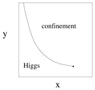
Figure 2: Schematic phase diagram of the Higgs model Eq. (4.1). Pure gauge theory is reached in the limit $x,y\rightarrow\infty$.

The phase diagram of the theory has been determined non-perturbatively in the continuum limit and is shown schematically in Fig. 2: Higgs and confinement regions are separated by a line of first order phase transitions, which ends in a critical point [21]. The spectrum in the respective regions as well as its continuous connection through the crossover region has been studied extensively [22, 23].

In the Higgs region, the theory has a physical vector boson carrying the quantum numbers of the gluon, coupling to the gauge invariant composite operator

$$W_{i}^{a}(x) = {\rm Tr\,}\left(T^{a}\Phi^{\dagger}(x)D_{i}\Phi(x)\right)\hskip 42.67912pt\mbox{(continuum)},$$

$$W_{i}^{a}(x) = {\rm Tr\,}\left(T^{a}\Phi^{\dagger}(x)U_{i}(x)\Phi(x+\hat{\i})\right)\quad\mbox{(lattice)}.$$ (4.3)

Its mass is determined by the decay of the corresponding correlation function

$$\langle W_{i}^{a}({\bf x},0)W_{i}^{a}({\bf x},t)\rangle\sim{\rm e}^{-M_{V}t}.$$ (4.4)

$M_{V}$ is an eigenvalue of the Hamiltonian acting on the gauge invariant subspace ${\cal H}$, and the W-boson is an asymptotic particle state. On the other hand, in perturbation theory one fixes a gauge and computes the vector boson mass from the fall-off of the gauge field propagator,

$$\langle A_{i}^{a}({\bf x},0)A_{i}^{a}({\bf x},t)\rangle\sim{\rm e}^{-m_{A}t}\ .$$ (4.5)

In momentum space the mass corresponds to the renormalized pole of the propagator. At a finite order in perturbation theory one finds $m_{A}=M_{V}$. With our operator constructed in the last section, Eq. (3.11), we now have a lattice implementable gauge field correlator without any reference to the scalar fields. We non-perturbatively know it to decay exponentially, where $m_{A}$ is an eigenvalue of the Hamiltonian acting on the entire Hilbert space ${\cal H}_{0}$.

Fig. 3 shows a comparison of the ground state mass as obtained from the two correlation functions, measured at one point in the Higgs phase, $x=0.0239,y=-0.02$, for different lattice spacings. Lattice sizes were chosen large enough for the masses to be free of finite volume effects, based on the results of [22]. Within statistical errors, the two operators yield identical results. The mass extracted from the new operator indeed extrapolates to a physical continuum limit, as promised in Sec. 3. As expected for an object with dimension $mass^{2}$, the lowest eigenvalue of the spatial covariant Laplacian diverges strongly in the continuum limit. For the correlation function this does not matter because the eigenvalue itself does not enter the definition of the correlation function.

      

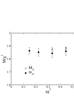
Figure 3: Left: The W-boson mass in a 3d Higgs phase, computed from the gauge invariant composite operator $W_{i}^{a}[\phi,U]$, Eq. (4.3), and the gauge field propagator, Eq. (3.11). The data for $M_{V}$ are from [22]. Right: The lowest eigenvalue of the lattice Laplacian, Eq. (3.1).

We then conclude that the gauge field propagator has a non-perturbative pole in the Higgs region of the model, and within our accuracy we find $m_{A}=M_{V}$ also non-perturbatively. While this may not be surprising, we stress that it is a non-trivial result. What has been known is that the perturbatively defined pole in the field propagator gives a good approximation of the physical W-mass in suitable gauges and when the perturbative Higgs expectation value is large compared to quantum fluctuations [24, 25], i.e. when perturbation theory is reliable. However, it has not been clear whether this pole also exists non-perturbatively, since that requires a non-perturbative definition for $m_{A}$. Moreover, it is important to realize that, because of the residual gauge freedom in the composite fields, Eq. (3.4), we have

$$\left\langle A^{a}_{i}[U]\;W^{a}_{i}[\phi,U]\right\rangle=0,$$ (4.6)

i.e. the operators are orthogonal, and so are the corresponding eigenstates of the Hamiltonian. This is yet another reflection of the fact that the eigenstates of the Hamiltonian $\hat{H}_{0}$ contributing to the correlator Eq. (3.11) are in a different sector of the Hilbert space than the eigenstates contributing to the correlator Eq. (4.4). Consequently, $m_{A},M_{V}$ are really different eigenvalues of $\hat{H}_{0}$ which are degenerate in a Higgs dynamics only.

The analytic connectedness of the phase diagram implies that there is a one to one mapping of the the entire spectrum of the Hamiltonian $\hat{H}_{0}$ between Higgs and confinement regions of the phase diagram [26]. For example, the W-boson state described by the operator Eq. (4.3), being an eigenstate of the projected transfer matrix $\hat{T}$, becomes a vector meson bound state in the confinement region [22, 23]. As we shall see, $m_{A}\neq M_{V}$ in a confining regime, as is also found in resummed perturbation theory [25, 27] and in lattice Landau gauge [28]. The parameters can be continuously tuned to $x,y\rightarrow\infty$, where the scalar fields are infinitely heavy and decouple to leave us with a pure gauge theory. All meson states including $M_{V}$ disappear from the (finite) spectrum in this limit. The question then is what happens to the pure gauge quantity $m_{A}$.

4.2 Yang Mills theory

In addition to a gluon, one may also construct other operators from the composite links Eq. (3.4). In particular, simply taking the trace,

$$O_{V}(x)={\rm Tr\,}(V_{i}(x)),$$ (4.7)

produces an operator coupling to $0^{++}$ states. It is fully invariant under gauge transformations, the residual freedom $h$ in the definition of the composite link discussed in Sec. 3 drops out under the trace. Hence, the correlation $\langle{\cal O}_{V}(x){\cal O}_{V}(y)\rangle$ falls off with the spectrum of the projected Hamiltonian $\hat{H}$, and one expects to be able to extract the $0^{++}$ glueball mass from it.

Fig. 4 shows the masses in lattice units extracted from the correlators in the $0^{++}$ and $1^{--}$ channels, respectively, plotted against the spatial length of the lattice, $L$. At intermediate and large distances we see a linear rise with $L$, which is reminiscent of torelons, i.e. flux loop states winding around the lattice [29]. The well-known $0^{++}$ torelon couples to Polyakov loops $P_{i}^{(L)}(x)=\prod_{n=0}^{L-1}\,U_{i}(x+n{{\hat{\imath}}})$, winding around a spatial direction of the lattice. Its mass extracted from the corresponding correlation function is related to the string tension in a finite volume,

$$\left\langle{\rm Tr\,}P_{i}^{(L)}({\bf x},0)\;{\rm Tr\,}P_{i}^{(L)}({\bf x},t)\right\rangle\simeq{\rm e}^{-am_{P^{(L)}}t},\quad am_{P^{(L)}}=a^{2}\sigma_{L}L.$$ (4.8)

Torelons are physical states in the gauge invariant sector in a finite volume, but become infinitely heavy and decouple when the infinite volume limit is taken. As Fig. 4 demonstrates, the two operators $O_{V},{\rm Tr\,}P^{(L)}$ give identical results and we conclude that $O_{V}$ projects onto the torelon.

Figure 4: Effective masses of $1^{--}$ and $0^{++}$ operators using the composite link $V[U]$ and Polyakov loops, as described in the text. The simulation is in YM-theory at $\beta=9$ with spatial lattice size $L$.

This suggests to interpret the lower $1^{--}$ state as torelonic state as well. In order to confirm this, we compare with the traceless part of the Polyakov loop. The latter is not gauge invariant, but if we replace the spatial link by a spatial Polykov loop, $U_{i}\rightarrow P_{i}^{(L)}$ in Eq. (3.4), the correlator Eq. (3.11) is again gauge invariant. The resulting masses are also shown in the plot and found to be identical to the ones from the original correlator. Hence we conclude that we have found a new eigenstate of the Hamiltonian for a pure gauge theory in a finite volume, corresponding to a torelon in an adjoint state. Because it transforms non-trivially, it is not an asymptotic state like the standard torelon, but rather an eigenstate of $\hat{H}_{0}$.

For $L=24$, we have also calculated the correlators with an $\Omega[U]$ computed from the Coulomb gauge fixing condition Eq. (3.13). As Fig. 4 shows, the results are, in accordance with our theoretical considerations, equivalent to those obtained from the Laplacian procedure. In particular, since the $\Omega$ emerging in Coulomb gauge is also non-local, it projects on the same winding states. The small deviation observed in the $1^{--}$ mass might be related to the influence of Gribov copies.

Fig. 4 is essentially unchanged when computed in the confining regime of the Higgs model rather than in the pure gauge theory. This is in agreement with previous findings that the confining gauge sector of the Higgs model is almost insensitive to the presence of the scalar fields [22, 23]. It confirms that the gluon correlator Eq. (3.11) does not project on the vector meson with mass $M_{V}$, but rather on a pure gauge quantity.

4.3 Localized vs. torelon states

Does the adjoint torelon state have anything to do with the gluon? For finite $L$ this is not the case, just like the $0^{++}$ torelon is not related to the glueball. The analytic connectedness of the phase diagram holds for the theory in infinite volume. This implies that the infinite volume pole in the gluon correlator found in the Higgs regime cannot disappear from the spectrum when the parameters are changed to the confining regime.

The reason for seeing only torelonic states is a projection problem of the maximally non-local operators: the functional $\Omega[U]$ depends on all links in the spatial volume. In a Higgs regime this is of no import because colour is screened and the links far from each other do not communicate. In a confining regime on the other hand, adjacent links form flux tubes stretching over the whole spatial lattice. An operator constructed from $\Omega$ must have a large overlap with such non-local objects, and a very small overlap with localized states. Put in another way, in the composite gauge field the link to be correlated, $U_{i}(x)$, is “drowned” by the dynamics of all other links contributing through $\Omega[U]$, a situation that worsens as the spatial volume is increased. For example, at some $L$ the $0^{++}$ torelon becomes heavier than the lightest glueball, which then should dominate the correlation function of $O_{V}$. At the lattice spacing chosen in Fig. 4, the lightest glueball mass is $aM_{G}=0.755(7)$ [31]. At $L=32$ the torelon is heavier, yet Fig. 4 demonstrates that $O_{V}$ is blind to the localized glueball state.

This finding is corroborated by the fact that the problem is absent when correlations other than those of pure gauge operators are studied. For example, propagators of an adjoint scalar field $\Phi(x)$ coupled to the gauge fields have been studied in the Coulomb gauge in [20]. No significant finite volume dependence was found for the scalar propagator. While the corresponding composite operator $\Omega^{\dagger}\Phi(x)\Omega(x)$ also employs a non-local function $\Omega[U]$, it is local in the scalar field to be correlated.

We then conclude that pure gauge operators constructed from the composite links $V_{i}$ in a confining dynamics have very weak overlap with localized states, and in their current form are not very useful to extract infinite volume physics. Nevertheless, a new eigenvalue of the Hamiltonian in the sector with quantum numbers of the gluon has been found. Just like the $0^{++}$ torelon is related to the potential of static charges in a singlet state, the adjoint piece of the flux tube should be related to the potential of static charges in a triplet state (octet for SU(3)) [32, 33]. This question is beyond the scope of the present paper and will be pursued elsewhere. However, having extracted the energy of a flux tube in an adjoint state, note that it extrapolates to a non-zero value $\sim 0.32g^{2}$ for $L\rightarrow 0$. In our Hamiltonian considerations we have interpreted the gluon mass as the minimal energy of precisely such a piece of flux. However, one would expect this value to be affected by finite volume effects, as one side of the lattice has been shrunk to zero.

5 The gluon mass and static mesons

In order to circumvent the projection problem encountered in the previous section, we now seek to compute the energy eigenvalue of interest from local observables coupled to sources. Rather than averaging over all their positions, the contribution of the sources will be computed separately and subtracted. This approach will also provide a relation between the gluon propagator in temporal gauge and the ratio of static meson correlators, leading to a physical interpretation of the gluon mass in terms of level splittings.

For this purpose we go back to the expressions of a gluon coupled to external sources in the continuum, Eq. (A1.8) from Appendix A, and on the lattice, Eq. (3.7). For a non-perturbative evaluation, we want to avoid the non-local functions used in the definition of the composite lattice gauge field. This may be achieved by observing that the energies governing the decay of a correlator are completely determined by the Hamiltonian and the quantum numbers of the operators. Instead of discretizing the gauge field, we may then equally well employ a local higher dimension operator sharing the same quantum numbers, such as the adjoint part of the linear combination of plaquettes in the spatial plane transverse to the Wilson line,

$${\cal O}_{DF}(x)=P_{i,j}(x)+P_{-i,j}(x)+P_{-j,-i}(x)+P_{-j,i}(x)-{\rm h.c.}$$ (5.1)

In the continuum limit, the operator approaches the covariant derivative of the field strength, $D_{j}F_{ij}(x)$, and couples to $J^{PC}=1^{--}$ states. We are then considering the two-point function

$$\langle{\cal O}^{a}({\bf x},0)U_{0,ab}^{A}({\bf x};0,t){\cal O}^{b}({\bf x},t)\rangle\sim{\rm e}^{-M_{{\cal O}}t},$$ (5.2)

with an adjoint temporal Wilson line $U_{0,ab}^{A}({\bf x};0,t)$. It has the general form of a gluelump correlator, describing a bound state of dynamical glue and a static adjoint source [18]. Hence we are looking for the mass of the lightest $1^{--}$, or “electric”, gluelump.

Because we are now working with undressed temporal links rather than with composite ones, the zero momentum projection Eq. (3.10) cannot be applied, and the observable still contains the divergent contribution from the adjoint Wilson line and its self-energy. We now need to compute this contribution separately and subtract it in order to get a finite result in the continuum limit. The Wilson line can be made gauge invariant by closing it through the periodic boundary in the $t$-direction, in which case it becomes an adjoint Polyakov loop, whose exponential decay with the temporal lattice size $N_{t}$ we need to compute. On the other hand, the Polyakov loop couples to adjoint states in all $J^{PC}$ sectors, and asymptotically its exponential decay is the same as that of Eq. (5.2), where ${\cal O}(x)$ is the operator leading to the smallest coefficient $M_{{\cal O}}$. Hence, we are looking for the mass of the lightest gluelump, which is well known [18] to be the “magnetic” one described by the clover field,

$${\cal O}_{F}(x)=P_{i,j}(x)+P_{j,-i}(x)+P_{-i,-j}(x)+P_{-j,i}(x)-{\rm h.c.}$$ (5.3)

In the continuum, this operator approaches the field strength $F_{ij}(x)$, coupling to $0^{--}$ and $1^{+-}$ states in 2+1 and 3+1 dimensions, respectively.

The lowest eigenvalue of $\hat{H}_{0}$ determining the asymptotic decay of the gluon correlation function Eq. (3.11) should then be the same as the gluelump mass splitting

$$m_{A}=M_{DF}-M_{F}\;.$$ (5.4)

Note that the gluelump states may be viewed as the zero distance limit of static potentials with the string between the sources being in an excited state specified by appropriate quantum numbers [18]. This is in accordance with our interpretation of the gluon mass as a short distance property of potentials put forward in the Hamiltonian strong coupling analysis, Sec. 2. The calculation of gluelump splittings involves only pure gauge operators local in space and is straightforward to evaluate on a lattice, with well controllable infinite volume and continuum limits.

5.1 Numerical result for SU(2) in 2+1 dimensions

Gluelumps in three dimensions have been simulated previously in different contexts [34, 35]. Here we are specifically interested in a continuum extrapolation of the mass splitting $M_{DF}-M_{F}$. The numerical results of a calculation in SU(2) pure gauge theory close to the continuum are displayed in Fig. 5. The choice of lattice sizes follows the results of [35], where it has been explicitly checked that the lowest gluelump is free of finite volume effects.

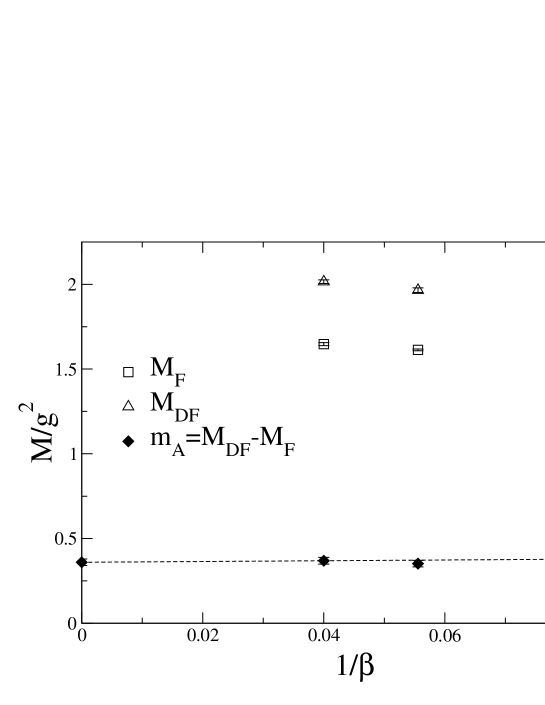
Figure 5: Masses for the electric ($M_{DF}$) and magnetic ($M_{F}$) gluelumps, as well as their mass splitting. Calculations have been performed for $\beta=12,18,25$ on lattices with $L=30,48,64$, respectively. The mass splitting is extrapolated to the continuum.

The figure displays the onset of the weak logarithmic divergence in the gluelump masses, as well as the expected scaling for their mass difference. A linear extrapolation of the data in $1/\beta$ to the continuum then gives the final result for the SU(2) gluon mass in 2+1 dimensions

$$m_{A}=0.360(19)g^{2},\qquad\chi^{2}/{\rm dof}=0.47.$$ (5.5)

Comparing with the lightest scalar glueball, $M_{G}=1.584(17)g^{2}$ [31], one finds $M_{G}/m_{A}=4.4(3)$.

5.2 The magnetic mass

Besides being an interesting test case, the gauge theory in 2+1 dimensions plays an important role in four-dimensional physics at finite temperature. Representing the Matsubara zero mode sector of the latter, it constitutes the effective theory describing all static physics at asymptotically high temperatures. A long standing problem of thermal field theories are the severe infrared divergencies encountered in perturbation theory. In particular, loops of magnetic gauge fields $A_{i}$ exhibit divergences on the three-dimensional scale $g^{2}\sim g_{4d}^{2}T$. These may be cured by dynamical generation of a “magnetic mass” which, however, is entirely non-perturbative and receives contributions from all orders in a loop expansion [36]. Here we have shown that such a magnetic mass can indeed be defined non-pertubatively, and that for hot SU(2) gauge theory its asymptotic high temperature value is $m_{A}=0.36(2)g_{4d}^{2}T$.

	ref.		$m_{A}/g^{2}$
1-loop gap eq.	[37]		0.38
	[27, 38]		0.28
	[39]		0.25
2-loop gap eq.	[40]		0.34
lattice MAG	[42]		0.51(6)

Table 1: Comparison of magnetic mass values from gap equations and gauge fixed lattice simulations.

In the past, gauge invariant resummation schemes have been designed to compute the pole of the gluon propagator self-consistently in three dimensions [27],[37]-[40]. In a Hamiltonian analysis of the three dimensional gauge theory a gauge invariant composite gluon variable has been constructed, which in the weak and strong coupling limits yields a gluon mass gap as the lowest eigenvalue of the Hamiltonian [41]. One may now compare the results of these approaches collected in Table 1 with the full answer and get an estimate for the quality of the approximations involved. It appears that the resummations lead to reasonable answers. In particular the two-loop result exhibits convergence towards the result of the last section. Note that lattice simulations employing maximal abelian gauge fixing provide numbers that are somewhat off our result, underlining the difficulty of obtaining stability in such calculations. In Landau gauge the correlator becomes negative at large distances, and it appears difficult to extract a mass [20].

5.3 Numerical result for SU(3) in 3+1 dimensions

The considerations to relate the gluon mass in pure gauge theory to the splitting of magnetic and electric gluelumps are directly applicable to SU(3) Yang-Mills theory in 3+1 dimensions. The only difference is that the lowest magnetic gluelump and the corresponding operator in four dimensions has $J^{PC}=1^{+-}$. The mass splitting between these lowest states has been computed in [10], which quotes for the continuum extrapolation

$$m_{A}=M_{DF}-M_{F}=368(7){\rm MeV}.$$ (5.6)

Comparing with the lightest scalar glueball, $M_{G}[0^{++}]=1730(130)$ MeV [43], we then have $M_{G}/m_{A}=4.7(5)$, which is strikingly similar to our 2+1 dimensional calculation in SU(2). This is not unexpected, given the close resemblance of other properties of pure gauge theories in 2+1 and 3+1 dimensions. Together with the ratio $M_{G}/m_{A}$, Table 2 collects results for the mass of the lightest scalar glueball and the string breaking distance for the flux tube between adjoint sources, suggesting that the confining low energy physics is very similar in these theories.

Similar to the situation in three dimensions, a larger value $m_{A}\approx 600$ MeV has recently been estimated from the gluon propagator in Laplacian gauge [45]. However, while this gauge is free from Gribov copies, no positive transfer matrix exists and hence the functional form of the decay is not exactly known.

Table 2: Comparison of some continuum extrapolated pure gauge quantities between 2+1 and 3+1 dimensions.

	2+1		3+1
SU(2), $M_{G}[0^{++}]/\sqrt{\sigma}$	4.	72(4) [31]	3.	74(12) [44]
SU(3), $M_{G}[0^{++}]/\sqrt{\sigma}$	4.	33(4) [31]	3.	64(9) [44]
SU(2), $M_{G}r^{adj}_{break}$	10.	3(1.5) [7]	$\sim$ 9.	7 [8]
SU(2), $M_{G}/m_{A}$	4.	4(3)	—
SU(3), $M_{G}/m_{A}$	—		4.	7(5) [43, 10]

6 Mass splittings between heavy mesons

In this section we ask what happens in the vicinity of the static limit, when heavy but dynamical matter fields are present, and whether the static limit can be attained smoothly. One might hope that the gluon mass is then observable in the spectrum of sufficiently heavy mesons. Two candidate splittings appear as possibilities.

First, hybrid meson states are, in the non-relativistic approximation, bound states in gluonic excitations of the static potential. These potentials have been calculated [46], and in the limit of small distances appear to smoothly connect to the gluelump spectrum [10]. In view of this the splitting of the lowest $1^{--}$ and $1^{+-}$ hybrid mesons, computed in the appropriate potentials, should be close to the gluon mass. However, these states have so far been elusive experimentally.

The second possibility is a splitting between a hybrid and a non-hybrid state. Since spin effects are suppressed, let us consider QCD with scalar quarks as specified in Appendix A. We are interested in the correlator of the vector meson

$$V_{i}(x)=\mathop{\rm Im}\left(\phi^{\dagger}(x)U_{i}\phi(x+\i)\right),\quad J^{PC}=1^{--},$$ (6.1)

but now we wish to keep the bare scalar mass $m_{0}$ finite rather than integrating over the scalar fields analytically. The main difference to the static case concerns the subtraction of the contribution of the scalar fields. Away from the static limit they will not sit at the same point in an adjoint state, but rather form spatially extended singlet mesons, the lightest of which couples to

$$S(x)=\mathop{\rm Re}\left(\phi^{\dagger}(x)\phi(x)\right),\quad J^{PC}=0^{++}.$$ (6.2)

Comparing the operator content of $S,V$, one may think of $V$ as a hybrid meson. The energy difference between vector and scalar mesons is accounted for by three different contributions: i) the total spin ${\bf J}={\bf L}_{\phi}+{\bf J_{g}}$, consisting of angular momentum of the scalars and the gluon spin; excitation of the ii) scalar and iii) gluon fields in higher quantum states. In the limit $m_{0}\rightarrow\infty$ the scalars become static and hence their angular momentum is switched off. Furthermore, they are “quenched” to be external fields and cannot be excited into higher quantum states. The remaining contributions to the mass splitting are the gluon spin and excitations of the gluon field. In this case the vector meson becomes spin-exotic, i.e. its quantum numbers cannot be accounted for without gluon degrees of freedom. Thus, the mass difference between vector and scalar meson in the static limit is probing a gluonic excitation with the quantum number of the gluon. This suggests that the gluon mass should be approached arbitrarily accurately by the limit

$$m_{A}=\lim_{m_{0}\rightarrow\infty}[M_{V}-M_{S}].$$ (6.3)

If the limit exists, the last equation may even serve as an alternative definition of the gluon mass. However, formally it is not clear whether a smooth limit exists. Calculating the scalar correlator in the static limit in the continuum using Eqs. (A1.3),(A1.5), one obtains

$$\langle S(x)S(y)\rangle\stackrel{{\scriptstyle m_{0}\rightarrow\infty}}{{\longrightarrow}}g_{0}^{2}(x,y)\left\langle{\rm Tr\,}\left(U_{0}(x,y)U^{\dagger}_{0}(x,y)\right)\right\rangle\;,$$ (6.4)

which has the same form on the lattice. The temporal Wilson lines combine to a unit matrix, hence the desired cancellation of their renormalization with that of the $V$ correlator does not work and, strictly speaking, the formal static limit of $M_{V}-M_{S}$ does not have a finite continuum limit. The reason is that static sources in a singlet state annihilate when they are at the same point. The only way for them to exist at zero separation is to combine their colour into an $(N^{2}-1)$-plet state, which we have used in the previous sections to calculate the static limit. However, this problem is absent for arbitrarily large but finite $m_{0}$, and one may ask whether the value for the gluon mass can be smoothly approached by $M_{V}-M_{S}$ for arbitrarily large $m_{0}$. As we shall see in the next section, this is indeed the case in 2+1 dimensions.

6.1 Heavy mesons for SU(2) in 2+1 dimensions

We now turn to a test of this proposition in the SU(2) lattice gauge theory in 2+1 dimensions. The scalar QCD action Eq. (A1.1) can then be rewritten in terms of scalar $2\times 2$ matrix fields $\Phi(x)$ and discretized as given in Appendix B. Results of detailed simulations for varying scalar mass $m_{0}$ are shown in Fig. 6, which displays the scalar and vector mesons, together with the lightest scalar glueball and its first excitation.

Note that scalar glueballs and mesons are indistinguishable by quantum numbers. To tell one from another a mixing analysis following [22, 23] has to be performed. Quite generally, the glueballs and scalar mesons show very little mixing even when they are close in mass, and thus are easy to identify. An example is shown in Fig. 6 (right), where the matrix elements between the $0^{++}$ mass eigenstates $\Psi_{n}$ and the operators used in the simulation ${\cal O}_{i}$ are displayed for $m_{0}=1.0g^{2}$. Here the operators are “smeared” versions of pure gauge and scalar operators, ${\cal O}_{i}\in\{G={\rm Tr\,}F_{ij}^{2},S=\phi^{\dagger}\phi\}$. (For details of the mixing analysis in a Higgs model, cf. [22]). Beginning with the lowest one, the three $0^{++}$ states are easily identified as glueball, scalar bound state and glueball, based on their operator content, and the situation is similar for the other parameter values.

The dotted error bands in Fig. 6 (left) give the location of the lightest scalar glueballs in the pure gauge theory [31]. It has already been reported for various scalar gauge models in 2+1 dimensions that the glueball spectrum deviates only at the percent level from that in the pure gauge theory [22, 23, 47]. Indeed the figure shows that already for bare masses $m_{0}\mathop{\raise 1.29167pt\hbox{$>$\kern-7.5pt\raise-4.73611pt\hbox{$\sim$}}}2g^{2}$ the glueball spectrum assumes its pure gauge values to high numerical accuracy, indicating that the scalars have largely decoupled as dynamical fields.

     

Figure 6: Left: The lowest states in 3d scalar QCD, simulated at $\beta=18$ on $48^{3}$ lattices. $M_{G}$ denotes scalar glueballs, $M_{S,V}$ scalar and vector mesons.
Right: Overlap $\langle\Psi_{i}|{\cal O}_{j}|0\rangle$ between the three lowest states $\Psi_{i}$ in the $0^{++}$ channel and blocked operators, ${\cal O}_{j}\in\{S,G\}$.

Also shown is the mass splitting between vector and scalar mesons, which is only slightly diminishing over the range of $m_{0}$ studied here. This is in accordance with the fact that we are close to the pure gauge limit. Note however, that in three dimensions the Coulomb part of the static potential is logarithmic. In a logarithmic potential, the level splittings of bound states of scalars calculated from a non-relativistic Schrödinger equation are also independent of the constituent mass [48], so that constancy of the splitting alone in this case cannot indicate the vicinity of the pure gauge limit.

According to the prescription Eq. (6.3), extracting the gluon mass requires an extrapolation of the splitting to infinite scalar masses. However, for heavier scalar fields the numerical errors grow rapidly and an accurate determination of the mass difference is increasingly difficult. This is well known from heavy quark physics and can in principle be cured by NRQCD methods [49]. Taking the largest value of $m_{0}$ in Fig. 6 one reads off $m_{A}=0.37(6)$. This is in excellent agreement with the static limit calculated in Sec. 5.1. We then conclude that in scalar QCD in 2+1 dimensions the gluon mass is observable to good accuracy in the mass splitting between vector and scalar mesons, which smoothly connects to the static limit.

6.2 Heavy quarkonia in QCD

Similar to the pure gauge physics in Table 2, a close resemblance is known between the SU(2) Higgs models in 2+1 and 3+1 dimensions. Both phase diagrams are analytically connected, with mass spectra of Higgs and W-bosons or bound states of scalars and glueballs in the Higgs and confinement regions, respectively (for a review and references, see [50]). Moreover, in the symmetric region the confinement and screening of fundamental charges as well as the mixing properties of the gluonic flux with meson states are the same in both models [51], and one might expect the results of the previous section to carry over. However, there is also a significant difference concerning the short range Coulomb part of the static potential, which is now $\sim r^{-1}$. While a calculation analogous to the one in Sec. 6.1 is beyond the scope of the current paper, it is intriguing to speculate about the situation in QCD, which provides us with heavy quarks to probe the gluon dynamics.

We then consider the mass splitting of heavy quarkonia instead of scalar mesons. Away from the static limit the situation is complicated by the quark spins, the total meson spin now being ${\bf J}={\bf L}_{q}+{\bf J}_{g}+{\bf S}_{q}$. Spin independent meson masses analogous to the case of heavy scalar fields (and static sources) are obtained by averaging over the quark spin multipletts. In the standard spectroscopic notation (based on the quark model) the total meson spin is written as ${\bf J}={\bf L}+{\bf S}_{q}$. Hence ${\bf L}={\bf L}_{q}+{\bf J}_{g}$, which is now playing the role of ${\bf J}={\bf L}_{\phi}+{\bf J}_{g}$ in the scalar case. Thus, based on a comparison of quantum numbers, the splitting $M_{V}-M_{S}$ in the theory with heavy scalars might correspond to the well known spin averaged mass splitting $\Delta_{1P-1S}$, as put forward in a preliminary account of this work [52]. Using current experimental numbers [53] one finds $\Delta_{1P-1S}(\bar{c}c)=418.5$ MeV and $\Delta_{1P-1S}(\bar{b}b)=416$ MeV.

However, it is not clear that these numbers are tied to the gluon mass. The fact that they are practically identical and quark mass independent cannot be taken as an indication of the proximity of the static limit, but is also accounted for by the effectively logarithmic non-relativistic bound state potential at the length scales relevant for these quarkonia [48, 54]. Increasing the quark mass pushes the states into the $\sim r^{-1}$ Coulomb region of the potential, in which mass splittings scale linearly with the quark mass. Hence the splittings of orbitally excited quarkonia do not have a static limit. On the other hand, this statement concerns only states within the non-relativistic quark model. In QCD there should be additional states, the hybrids, in which gluonic excitations account for the same quantum numbers, and one would expect the static limit of the splitting to exist. In general mixing analyses are necessary in order to unambiguously identify the nature of an observed state. A four-dimensional analogue of the calculation in Sec. 6.1 could clarify this question.

7 Conclusions

It has been demonstrated that an unambiguous, non-perturbative definition of a gluon mass is possible in terms of an eigenvalue of the Kogut-Susskind Hamiltonian of lattice gauge theory, which can be interpreted as the energy of a gluon coupled to static sources. This eigenvalue can be computed in several ways. It dictates the asymptotic exponential decay of non-local pure gauge observables which, in a particular gauge, reduce to the gauge field propagator. Using the eigenvectors of the covariant Laplacian for its construction, these observables are free of Gribov copies and strictly positive, with effective masses being upper bounds to the ground state. In practice these operators are numerically feasible in Higgs regimes, but not in confining dynamics, where their non-local nature results in an almost exclusive projection onto torelonic states.

However, the same eigenvalue also governs the asymptotic exponential decay of ratios of static gluelumps, in which gluon fields are bound to adjoint sources. This establishes a non-perturbative relation between the gluon mass and manifestly gauge invariant observables. These can be easily computed using local operators, with well controlled infinite volume and continuum limits. Furthermore, in three dimensions the mass splitting of vector and scalar mesons approaches the same quantity in the static limit. In four dimensions this might be modified due to the different nature of the Coulomb potential.

Viewing the lattice field theory as a statistical system, it is clear that this gluonic mass scale plays a fundamental role in colour dynamics: $1/m_{A}$ is the largest correlation length in the pure gauge system, providing an infrared cut-off for virtual states as well as setting a scale for the screening of colour interactions. For thermal physics, in particular, this should allow a non-abelian definition of Debye screening in complete analogy to QED. Moreover, the fact that $m_{A}$ in three dimensions is finite implies a non-zero magnetic mass which we have computed for SU(2), and thus the screening of colour magnetic fields in a plasma. A physical interpretation of the zero temperature gluon mass requires more work to investigate the static limit of meson mass splittings.

We then conclude that a general gauge invariant description of colour dynamics in terms of partonic degrees of freedom should be possible, with numerous interesting questions to be answered. First, it would be very desirable to solve the projection problem of the non-local gluon propagators and numerically confirm the relations between their exponential decay and the static mesons established here. An obvious generalization would be to apply the same techniques to quark propagators, which might offer an alternative approach to non-perturbative quark mass renormalization. Similar methods applied to Polyakov loops should also allow to give a gauge invariant meaning to the finite temperature static potential with sources in an octet state. Finally, one may hope to get a new handle on some proposed confinement mechanisms. For example, a gluon getting massive dynamically is in acccord with what is expected in a picture of the vacuum as a dual superconductor.

Appendix A Continuum pure gauge theory with static sources

Let us introduce a complex scalar $N$-plet $\phi_{\alpha}(x)$, $\alpha=1,...N$, coupled to the gauge fields, with the action

$$S_{\phi}[A,\phi]=\int d^{3}x\;\left\{(D_{\mu}\phi)^{*}(x)D_{\mu}\phi(x)+m_{0}^{2}\phi^{*}(x)\phi(x)\right\}.$$ (1.1)

Together with the pure gauge action, the theory corresponds to QCD with scalar “quarks”. In the limit $m_{0}\rightarrow\infty$ the terms $|D_{i}\phi|^{2}$ are suppressed and decouple from the above action. In this case the scalar fields propagate in time only, describing static sources coupling to colour electric flux of the gauge fields. The scalar propagator satisfying $\left(-D_{0}^{*}D_{0}+m_{0}^{2}\right)G(x,y)=\delta(x-y)$ is known exactly:

$$G(x,y)=g_{0}(x,y)\delta({\bf x},{\bf y})U_{0}(x,y),$$ (1.2)

where $g_{0}(x,y)$ is the free scalar propagator without background field and $U_{0}(x,y)$ the temporal Wilson line from $x$ to $y$.

We are interested in observables of the type ${\cal O}(x_{1},x_{2})=\phi^{\dagger}(x_{1})M(x_{1},x_{2})\phi(x_{2})$, where $M(x_{1},x_{2})$ is a pure gauge matrix operator containing Wilson lines and/or covariant derivatives. Doing the Gaussian integral over the scalars one obtains for the correlation function ($x_{i}=({\bf x}_{i},0),y_{i}=({\bf x}_{i},t)$)

$$\langle{\cal O}(x_{1},x_{2}){\cal O}^{\dagger}(y_{1},y_{2})\rangle=Z^{-1}\int DA\;\;\bar{{\cal O}}[A]\;{\rm e}^{-S_{YM}[A]},$$ (1.3)

with

$$Z = \int DA\;Z_{\phi}\;{\rm e}^{-S_{YM}[A]},\quad Z_{\phi}=[\det(-D^{2}+m_{0}^{2})]^{-1},$$

$$\bar{{\cal O}}[A] = Z_{\phi}^{-1}\int D\phi D\phi^{*}\;{\cal O}(x_{1},x_{2}){\cal O}^{\dagger}(y_{1},y_{2})\;{\rm e}^{-S_{\phi}[A,\phi]}.$$ (1.4)

In the limit $m_{0}\rightarrow\infty$ the scalar determinant becomes a constant and $\bar{{\cal O}}[A]$ represents a pure gauge quantity,

$$\bar{{\cal O}}[A]=g_{0}(x_{1},y_{1})g_{0}(x_{2},y_{2})\;{\rm Tr\,}[M(x_{1},x_{2})U_{0}(x_{2},y_{2})M^{\dagger}(y_{1},y_{2})U_{0}(y_{1},x_{1})].$$ (1.5)

A prominent example is the string of colour flux ending on scalar charges separated by $r=|{\bf x}_{1}-{\bf x}_{2}|$, which is described by the operator $M(x_{1},x_{2})=U(x_{1},x_{2})$. In the limit $m_{0}\rightarrow\infty$ the correlator goes over into the Wilson loop,

$$\langle{\cal O}(x_{1},x_{2}){\cal O}(y_{1},y_{2})\rangle\stackrel{{\scriptstyle m_{0}\rightarrow\infty}}{{\longrightarrow}}g^{2}_{0}(t)\langle W(r,t)\rangle,$$ (1.6)

decaying exponentially with the energy of the string in the presence of sources.

In the same way as the energy of a flux tube, the gluon energy can be probed by coupling it to scalar sources. In making contact to the lattice strong coupling gluon wave function Eq. (2.10), we consider the simplest gauge invariant operator with $J^{PC}$ quantum numbers of the gluon,

$$V_{i}(x)=\mathop{\rm Im}\left(\phi^{\dagger}(x)D_{i}\phi(x)\right),\quad J^{PC}=1^{--}.$$ (1.7)

The connection to the gluon propagator is established by integrating over the scalars analytically. Using Eqs. (1.3),(1.5), one finds for the correlator

$$\langle V_{i}(x)V_{i}(y)\rangle\stackrel{{\scriptstyle m_{0}\rightarrow\infty}}{{\longrightarrow}}-g_{0}^{2}(x,y)\left\langle{\rm Tr\,}\left[D_{i}(x)U_{0}(x,y)D_{i}(y)U^{\dagger}_{0}(x,y)\right]\right\rangle.$$ (1.8)

Since the expression is manifestly gauge invariant, it may be evaluated in any gauge. Choosing the temporal gauge, $A_{0}(x)=0$, we have $U_{0}(x,y)=1$ and $D_{i}(x)U_{0}(x,y)\rightarrow-2igA_{i}(x)$, The right hand side of Eq. (1.8) is thus identical to the gluon propagator in temporal gauge times a free scalar propagator,

$$\lim_{m_{0}\rightarrow\infty}\langle V_{i}(x)V_{i}(y)\rangle\left.\right|_{A_{0}=0}=4g^{2}g_{0}^{2}(x,y)\left.\langle{\rm Tr\,}A_{i}(x)A_{i}(y)\rangle\right|_{A_{0}=0}.$$ (1.9)

Note that the pure gauge operator in Eq. (1.8) is simply the continuum version of Eq. (3.6). It is then clear that its exponential decay is determined by the spectrum of the continuum Hamiltonian in temporal gauge. However, in the continuum, $D_{i}(x)$ is an operator defined at a point, which allows its correlator to be written down without the introduction of non-local functions of the gauge field.

Appendix B Lattice actions

In this appendix we give the lattice action and parameters used for the simulations in the various parts of this paper.
SU(2) Higgs model, Sec. 4.1: The lattice action for the fundamental representation Higgs model in 2+1 dimensions with $2\times 2$ matrix field $\Phi(x)$, cf. Eq. (4.1), may be defined as

$$S[U,\Phi] = \beta\sum_{p}\left(1-\frac{1}{2}{\rm Tr\,}U_{p}\right)+\sum_{x}\Bigg{\{}-\beta_{H}\sum_{i=1}^{3}\frac{1}{2}{\rm Tr\,}\Big{(}\Phi^{\dagger}(x)U_{i}(x)\Phi(x+\hat{i})\Big{)}$$ (2.1)

$$+\frac{1}{2}{\rm Tr\,}\Big{(}\Phi^{\dagger}(x)\Phi(x)\Big{)}+\beta_{R}\left[\frac{1}{2}{\rm Tr\,}\Big{(}\Phi^{\dagger}(x)\Phi(x)\Big{)}-1\right]^{2}\Bigg{\}}.$$

The relation between the parameters of the continuum action Eq. (4.1) and those of the lattice action is at the two loop level [55]

$$\beta = \frac{4}{ag^{2}},$$

$$\beta_{R} = x\frac{\beta_{H}^{2}}{\beta},$$

$$y = \frac{\beta^{2}}{8}\left(\frac{1}{\beta_{H}}-3-\frac{2\beta_{H}}{\beta}x\right)+\frac{3\Sigma\beta}{32\pi}\left(1+4x\right)$$ (2.2)

$$+\frac{1}{16\pi^{2}}\left[\left(\frac{51}{16}+9x-12x^{2}\right)\left(\ln\frac{3\beta}{2}+\zeta\right)+5.0+5.2x\right]\;,$$

with the numerical constants $\Sigma=3.17591$ and $\zeta=0.09$. Due to superrenormalizability, Eq. (2.2) are exact up to discretization errors. The continuum limit is at one point in the lattice phase diagram, $\beta_{G}\rightarrow\infty,\beta_{H}=1/3,\beta_{R}=0$.
Yang-Mills limit, Secs. 4.2, 5.1: The pure gauge action is seen to be a limit of the above obtained by taking $\beta_{H}=\beta_{R}=0$. From Eq. (2.2) it is evident that this corresponds to sending the continuum parameters $x,y\rightarrow\infty$.
Scalar QCD, Sec. 6.1: Finally, the Gaussian scalar action simulated in Sec. 6.1 is obtained by taking $\beta_{R}=0$.

The algorithm used to perform the Monte Carlo simulation using the action in Eq. (2.1) is the same as in [22, 23]. The gauge variables are updated by a combination of heatbath and over-relaxation steps according to [56, 57], while the scalar degrees of freedom are updated combining heatbath and reflection steps as described in [58]. The ratio of the different updating steps is suitably tuned such as to minimize autocorrelations. In the simulations we gathered typically between 5 000 and 20 000 measurements taken after such combinations of updating sweeps.

In order to increase the overlap of operators with the low energy states to be measured, standard “smearing” or “blocking” techniques have been applied to gauge and scalar fields. The correlation matrix between operators of different smearing levels is measured and diagonalized by a variational calculation allowing to extract ground and excited states in a given quantum number channel. For details and references see [22].

References

- [1] R. Kobes, G. Kunstatter and A. Rebhan, Phys. Rev. Lett. 64 (1990) 2992; Nucl. Phys. B 355 (1991) 1.
- [2] A. S. Kronfeld, Phys. Rev. D 58 (1998) 051501.
- [3] J. E. Mandula and M. Ogilvie, Phys. Lett. B 185 (1987) 127.
- [4] V. N. Gribov, Nucl. Phys. B 139 (1978) 1; P. van Baal, hep-th/9711070.
- [5] L. Giusti, M. L. Paciello, C. Parrinello, S. Petrarca and B. Taglienti, Int. J. Mod. Phys. A 16 (2001) 3487.
- [6] C. W. Bernard, Nucl. Phys. B 219 (1983) 341.
- [7] O. Philipsen and H. Wittig, Phys. Lett. B 451 (1999) 146.
- [8] P. de Forcrand and O. Philipsen, Phys. Lett. B 475 (2000) 280.
- [9] O. Philipsen, Phys. Lett. B 521 (2001) 273.
- [10] M. Foster and C. Michael [UKQCD Collaboration], Phys. Rev. D 59 (1999) 094509.
- [11] J. Kogut and L. Susskind, Phys. Rev. D 11 (1975) 395.
- [12] M. Creutz, Phys. Rev. D 15 (1977) 1128.
- [13] M. Lüscher, Commun. Math. Phys. 54 (1977) 283.
- [14] J. C. Vink, Phys. Rev. D 51 (1995) 1292.
- [15] J. C. Vink and U. Wiese, Phys. Lett. B 289 (1992) 122.
- [16] G. Mack, T. Kalkreuter, G. Palma and M. Speh, hep-lat/9205013; U. Kerres, G. Mack and G. Palma, Nucl. Phys. B 467 (1996) 510.
- [17] C. Alexandrou, P. de Forcrand and E. Follana, Phys. Rev. D 63 (2001) 094504.
- [18] C. Michael, Nucl. Phys. B 259 (1985) 58; I. H. Jorysz and C. Michael, Nucl. Phys. B 302 (1988) 448.
- [19] G. C. Rossi and M. Testa, Nucl. Phys. B 163 (1980) 109.
- [20] A. Cucchieri, F. Karsch and P. Petreczky, Phys. Rev. D 64 (2001) 036001.
- [21] K. Kajantie, M. Laine, K. Rummukainen and M. E. Shaposhnikov, Phys. Rev. Lett. 77 (1996) 2887; K. Rummukainen, M. Tsypin, K. Kajantie, M. Laine and M. E. Shaposhnikov, Nucl. Phys. B 532 (1998) 283.
- [22] O. Philipsen, M. Teper and H. Wittig, Nucl. Phys. B 469 (1996) 445.
- [23] O. Philipsen, M. Teper and H. Wittig, Nucl. Phys. B 528 (1998) 379.
- [24] J. Fröhlich, G. Morchio and F. Strocchi, Nucl. Phys. B 190 (1981) 553.
- [25] W. Buchmüller and O. Philipsen, Phys. Lett. B 397 (1997) 112.
- [26] E. H. Fradkin and S. H. Shenker, Phys. Rev. D 19 (1979) 3682.
- [27] W. Buchmüller and O. Philipsen, Nucl. Phys. B 443 (1995) 47.
- [28] F. Karsch, T. Neuhaus, A. Patkos and J. Rank, Nucl. Phys. B 474 (1996) 217.
- [29] C. Michael, J. Phys. G 13 (1987) 1001.
- [30] P. de Forcrand, G. Schierholz, H. Schneider and M. Teper, Phys. Lett. B 160 (1985) 137.
- [31] M. J. Teper, Phys. Rev. D 59 (1999) 014512.
- [32] L. D. McLerran and B. Svetitsky, Phys. Rev. D 24 (1981) 450.
- [33] S. Nadkarni, Phys. Rev. D 34 (1986) 3904.
- [34] G. I. Poulis and H. D. Trottier, Phys. Lett. B 400 (1997) 358.
- [35] M. Laine and O. Philipsen, Nucl. Phys. B 523 (1998) 267; Phys. Lett. B 459 (1999) 259.
- [36] A. D. Linde, Phys. Lett. B 96 (1980) 289; D. J. Gross, R. D. Pisarski and L. G. Yaffe, Rev. Mod. Phys. 53 (1981) 43.
- [37] G. Alexanian and V. P. Nair, Phys. Lett. B 352 (1995) 435.
- [38] R. Jackiw and S. Pi, Phys. Lett. B 403 (1997) 297.
- [39] J. M. Cornwall, Phys. Rev. D 57 (1998) 3694;
- [40] F. Eberlein, Phys. Lett. B 439 (1998) 130; Nucl. Phys. B 550 (1999) 303.
- [41] D. Karabali and V. P. Nair, Phys. Lett. B 379 (1996) 141; D. Karabali, C. Kim and V. P. Nair, Nucl. Phys. B 524 (1998) 661.
- [42] A. Cucchieri, F. Karsch and P. Petreczky, Phys. Lett. B 497 (2001) 80.
- [43] C. J. Morningstar and M. J. Peardon, Phys. Rev. D 60 (1999) 034509.
- [44] M. J. Teper, Glueball masses and other physical properties of SU(N) gauge theories in D = 3+1: A review of lattice results for theorists, hep-th/9812187.
- [45] C. Alexandrou, P. d. Forcrand and E. Follana, arXiv:hep-lat/0112043.
- [46] S. Perantonis and C. Michael, Nucl. Phys. B 347 (1990) 854; K. J. Juge, J. Kuti and C. J. Morningstar, Nucl. Phys. Proc. Suppl. 63 (1998) 326.
- [47] A. Hart and O. Philipsen, Nucl. Phys. B 572 (2000) 243; A. Hart, M. Laine and O. Philipsen, Nucl. Phys. B 586 (2000) 443.
- [48] C. Quigg and J. L. Rosner, Phys. Rept. 56 (1979) 167.
- [49] B. A. Thacker and G. P. Lepage, Phys. Rev. D 43, 196 (1991).
- [50] I. Montvay and G. Münster, Quantum fields on a lattice, Cambridge Univ. Pr. (1994) 491 pp.
- [51] O. Philipsen and H. Wittig, Phys. Rev. Lett. 81, 4056 (1998) [Erratum-ibid. 83, 2684 (1998)]. F. Knechtli and R. Sommer [ALPHA Collaboration], Nucl. Phys. B 590, 309 (2000).
- [52] O. Philipsen, Non-perturbative parton mass for the gluon, hep-lat/0110114.
- [53] D. E. Groom et al. [Particle Data Group Collaboration], Eur. Phys. J. C 15 (2000) 1.
- [54] W. Buchmüller and S. H. Tye, Phys. Rev. D 24 (1981) 132.
- [55] M. Laine, Nucl. Phys. B 451 (1995) 484.
- [56] K. Fabricius and O. Haan, Phys. Lett. B 143 (1984) 459.
- [57] A.D. Kennedy and B.J. Pendleton, Phys. Lett. B 156 (1985) 393.
- [58] B. Bunk, Nucl. Phys. B (Proc. Suppl.) 42 (1995) 566.