A Lattice Study Of The Magnetic Moment
And The Spin Structure Of The Nucleon

Abstract

Using an approach free from momentum extrapolation, we calculate the nucleon magnetic moment and the fraction of the nucleon spin carried by the quark angular momentum in the quenched lattice QCD approximation. Quarks with three values of lattice masses, $210,~{}124$ and $80~{}{\rm MeV}$, are formulated on the lattice using the standard Wilson approach. At every mass, 100 gluon configurations on $16^{3}\times 32$ lattice with $\beta=6.0$ are used for statistical averaging. The results are compared with the previous calculations with momentum extrapolation. The contribution of the disconnected diagrams is studied at the largest quark mass using noise theory technique.

I Introduction

The magnetic moment is one of the fundamental properties of the nucleon. Experimentally this quantity has been measured to a very high precision [1]. In the nucleon model-building, the magnetic moment is usually the first to check against the experimental data. To understand how well a particular version of lattice QCD can simulate the internal structure of the nucleon, the magnetic moment is an observable that one must study after the nucleon mass.

Theoretical computations of the nucleon magnetic moment using lattice QCD techniques have been performed by a number of groups on lattices of different physical sizes and lattice spacings with different nucleon sources (interpolating fields) [2]-[7]. Most calculations done so far have used the quenched approximation. And almost all calculations begin with the lattice calculations of Sach’s magnetic form-factor $G_{M}(Q^{2})$, where $Q^{2}=-q_{0}^{2}+{\vec{q}}^{2}$, at discrete values of the momentum transfer $\vec{q}$. The magnetic moment is just $G_{M}(Q^{2})$ at $Q^{2}=0$ which can not be obtained more directly in this approach because the relevant off-forward matrix element is linearly proportional to ${\vec{q}}$. The lattice magnetic momentum is obtained usually by extrapolating these discrete values at finite $Q^{2}$ to $0$.

However, there are potential problems in the $Q^{2}$ extrapolation, mainly due to the finite volume effects. On a finite lattice, the momentum transfer ${\vec{q}}=(q_{1},q_{2},q_{3})$ is quantized: $q_{i}=2\pi\cdot n/N_{i}$ in unit of inverse lattice spacing, where $N_{i}$ is the total number of sites in momentum direction $i$ and $n=0,1,...,N_{i}$ is an integer. The smallest possible non-zero $Q^{2}$ is equal to $-q_{0}^{2}+(2\pi/{\rm Max}(N_{i}))^{2}$, where $q_{0}=\sqrt{M^{2}+(2\pi/{\rm Max}(N_{i}))^{2}}-M$, and $M$ is the nucleon mass. For a lattice with a spatial dimension $16^{3}$, $Q^{2}_{\rm min}=2M(\sqrt{(\pi/8)^{2}+M^{2}}-M)$. For $\beta=6$, this corresponds to $\sim 0.5~{}{\rm GeV}^{2}$. At this scale, the nucleon form factors are very sensitive functions of $Q^{2}$. Indeed $G_{E}(Q^{2})$ increases from $Q^{2}=0.5~{}{\rm GeV}^{2}$ to $Q^{2}=0$ by almost a factor of 3. Therefore, an extrapolation across this range of $Q^{2}$ must be strongly model dependent if without any prior knowledge of the $Q^{2}$ dependence of the nucleon form factors [4, 8, 9, 10]. Fortunately, the experimental data shows that the $Q^{2}$-dependence of the nucleon form factors can be fitted to a dipole form. Moreover, in a limited $Q^{2}$ range, the dipole form is not too different from a monopole. Therefore, we find in the literature both forms are commonly used to fit the lattice data [4, 10, 11]. An example of the extrapolation using different fitting formula can be found in Ref. [4].

In this paper, we report a more direct calculation of the nucleon magnetic moment using the elementary definition in electromagnetism [12]. Although this approach was first mentioned in Ref. [4], to our knowledge, however, no systematic study along this line has ever been reported in the literature. As is quite obvious, the great advantage of this method is that it is free from the extrapolation of the finite momentum transfer $Q^{2}$. We will comment on a different finite volume effect later in this paper.

Using a similar approach, we can calculate the fraction of the nucleon spin carried by the quark angular momentum. In recent years, the study of the spin structure of the nucleon has stimulated much interest in both the experimental and theoretical nuclear and particle community [13, 14]. It was found in Ref. [15] that the quark angular momentum in the nucleon can be obtained through deeply-virtual Compton scattering and other hard exclusive processes. While this observation has stimulated much perturbative QCD and phenomenological study [16], the quark angular momentum can also be calculated in lattice QCD. A first attempt in which the momentum extrapolation was used in the magnetic moment calculation was reported in Ref. [17]. As shown in Ref. [15], it can be calculated using the direct theoretical definition as well. In this paper, we also report such a calculation.

Our paper is organized as follows. In Sec. II, we give a brief theoretical discussion of the nucleon magnetic moment and quark angular momentum in the continuum. We state our conventions and describe the implementation of the continuum formulas in the lattice simulations. In Sec. III, we outline the setup of our lattice calculations and present our main results. We will compare them with previous calculations. We also consider the contributions of the disconnected diagrams to both the magnetic moment and quark total angular momentum. In the final section, we present the conclusion and discuss possible ways to improve upon the present calculation.

II Theoretical Details

In this section, we present a number of theoretical formulas which are useful in our numerical calculations. In the process, we will make clear our notations and conventions.

A Magnetic Moment and Quark Angular Momentum

According to the standard electromagnetic theory the magnetic moment operator of a system can be defined as [12]:

$${\vec{\mu}}={1\over 2}\int[{\vec{r}}\times{\vec{j}}_{\rm em}]d^{3}r\ ,$$ (1)

where $\vec{j}_{\rm em}$ is the electromagnetic current density. Its matrix element in a quantum state $|jm_{z}=j\rangle$ ($\langle jm|jm\rangle=1$) quantized in the $z$-direction defines the magnetic moment,

$$\mu=\langle jm_{z}=j|\hat{\mu}_{z}|jm_{z}=j\rangle\ .$$ (2)

We will use this definition to calculate the magnetic moment of the nucleon in its rest frame.

The magnetic moment can also be obtained from the form factors of the electromagnetic current. For the nucleon, we have [18]

$$\langle P^{\prime}S^{\prime}|j_{\rm em}^{\mu}(0)|PS\rangle=\overline{u}(P^{\prime}S^{\prime})\left[\gamma^{\mu}F_{1}(Q^{2})+i\frac{\sigma^{\mu\nu}q^{\nu}}{2m_{N}}F_{2}(Q^{2})\right]u(PS)\ ,$$ (3)

where $\sigma^{\mu\nu}=\frac{i}{2}[\gamma^{\mu},\gamma^{\nu}]$, $|PS\rangle$ represents the ground state of the nucleon with four-momentum $P$ and polarization $S$, $q=P^{\prime}-P$ is the momentum transfer, $Q^{2}=-q_{0}^{2}+{\vec{q}}^{2}$, and $u(PS)$ is an on-shell Dirac spinor. $F_{1}(Q^{2})$ and $F_{2}(Q^{2})$ are the well-known Dirac and Pauli form factors. The nucleon magnetic moment can be obtained from Sach’s magnetic form factor

$$G_{M}(Q^{2})=F_{1}(Q^{2})+F_{2}(Q^{2})$$ (4)

at $Q^{2}=0$: $\mu_{N}=G_{M}(0)$. This approach has been used in most of the lattice QCD calculations.

To understand the spin structure of the nucleon, one needs the QCD angular momentum operator in a gauge-invariant form [15, 14]

$${\vec{J}}_{\rm QCD}={\vec{J}}_{\rm g}+{\vec{J}}_{\rm q}\ ,$$ (5)

with

$${\vec{J}}_{\rm q} = \int d^{3}r[{\vec{r}}\times{\vec{T}}]=\int d^{3}r\left[\psi^{\dagger}\frac{{\vec{\Sigma}}}{2}\psi+\psi^{\dagger}[{\vec{r}}\times(-i\overrightarrow{D})]\psi\right]\ ,$$ (6)

$${\vec{J}}_{\rm g} = \int d^{3}r\left[{\vec{r}}\times[{\vec{E}}\times{\vec{B}}]\right]\ ,$$ (7)

where ${\vec{\Sigma}}$ is the Dirac spin matrix and $\overrightarrow{D}=\overrightarrow{\nabla}-ig{\vec{A}}$ is the covariant derivative, ${\vec{T}}=(T^{j0})$ is a component of the quark energy-momentum tensor to be defined later. In a nucleon state with helicity 1/2 and momentum along the $z$-direction, the total helicity can be calculated as the expectation value of $J_{z}$,

$$\frac{1}{2}=\frac{1}{2}\Sigma+L_{\rm q}+J_{\rm g}=J_{\rm q}+J_{\rm g}\ ,$$ (8)

where the various contributions to the spin of the nucleon are defined as the expectation values of the corresponding operators. For instance, the matrix element of ${\vec{J}}_{\rm q}$ defines the quark total angular momentum contribution to the nucleon spin.

As in the case of the nucleon magnetic moment, the quark contribution to the nucleon spin $J_{q}$ can be obtained from the form factors of the quark energy-momentum tensor $T^{\mu\nu}=\frac{i}{2}{\overline{\psi}}\stackrel{{\scriptstyle\leftrightarrow}}{{D^{(\mu}}}\gamma^{\nu)}\psi$ (the parentheses around the two indices means symmetrization and subtraction of the trace and $\stackrel{{\scriptstyle\leftrightarrow}}{{D}}=\stackrel{{\scriptstyle\rightarrow}}{{D}}-\stackrel{{\scriptstyle\leftarrow}}{{D}}$)

$$\langle P^{\prime}S^{\prime}|T^{\mu\nu}(0)|PS\rangle=$$ (9)

$$\overline{u}(P^{\prime}S^{\prime})\left[\overline{P}^{(\mu}\gamma^{\nu)}T_{1}(Q^{2})+\frac{\overline{P}^{(\mu}i\sigma^{\nu)\beta}q^{\beta}}{2M}T_{2}(Q^{2})+\frac{q^{(\mu}q^{\nu)}}{M}T_{3}(Q^{2})\right]u(PS)\ ,$$ (10)

where $\overline{P}^{\mu}=(P^{\mu}+P^{\prime\mu})/2$. The quark contribution to the spin of the nucleon is then simple $J_{\rm q}=\frac{1}{2}[T_{1}(0)+T_{2}(0)]$. In Ref. [17], this was used to calculate $J_{q}$.

B Lattice Formalism

Light (up and down) quarks are put on the lattice using the standard Wilson formulation. In the discrete Euclidean spacetime, the fermionic part of the QCD action is given by [19]:

$$S_{W}=\sum\limits_{i,j}\overline{\psi}_{i}M_{ij}\psi_{j}\ ,$$ (11)

where $i,j$ is the sum over the full set of spacetime, Dirac, color indices with $i=\{x,\alpha,a\}$ and $j=\{y,\beta,b\}$. $M_{ij}$ is defined as

$$M_{ij}=\delta_{i,j}-\kappa\sum\limits_{\mu}\left\{(1-\gamma_{\mu})_{\alpha\beta}U_{\mu}(x)^{ab}\delta_{x,y-\hat{\mu}}+(1+\gamma_{\mu})_{\alpha\beta}U^{\dagger}_{\mu}(x-\hat{\mu})^{ab}\delta_{x,y+\hat{\mu}}\right\}\ ,$$ (12)

where $\kappa=1/(2(m_{0}+4))$ with $m_{0}$ the bare quark mass, $\hat{\mu}$ is a unit vector along the $\mu=1,2,3,4$ direction, and the lattice spacing $a$ is set to 1. $U_{\mu}(x)=e^{iA_{\mu}(x)}$ represents a link connecting the nearest lattice sites going from $x$ to $x+\hat{\mu}$. Our notation for $\gamma$-matrices follows Refs. [20, 21]:

$$\gamma_{4}^{E}=\gamma^{0}=\pmatrix{I&0\cr 0&-I},\hskip 8.53581pt\gamma^{E}_{i}=-i\gamma^{i}=\pmatrix{0&-i\sigma_{i}\cr i\sigma_{i}&0}\ ,$$ (13)

where $E$ means Euclidean space and will be omitted henceforth. The standard continuum Dirac field $\psi$ is related to the above by an extra factor of $\sqrt{m_{0}+4}$.

We are interested in calculating two- and three-point correlation functions involving the nucleon interpolating fields on the lattice. The graphical representation for them is shown in Fig.1, where $t_{0}$ is the “time” of the nucleon creation (source position), $t_{x}$ is the “time” of the nucleon annihilation (sink position) and $t_{y}$ is the “time” of the operator insertion (we sum only over the spatial coordinates ${\vec{x}}$ and ${\vec{y}}$).

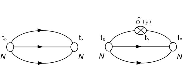
FIG. 1.: Two-point and three-point diagrams.

The nucleon two-point correlation function is defined as

$$G_{2\alpha\alpha^{\prime}}(t_{x},{\vec{P}^{\prime}})=\sum\limits_{\vec{x}}e^{-i{\vec{P}^{\prime}}{\vec{x}}}\langle 0|\chi_{\alpha}(x)\overline{\chi}_{\alpha^{\prime}}(0)|0\rangle\ ,$$ (14)

where $x=(t_{x},{\vec{x}})$ are discretized spacetime coordinates, $\alpha,\alpha^{\prime}$ are Dirac indices, and $|0\rangle$ represents QCD vacuum. Operator $\chi$ is an interpolating field with the nucleon quantum number. We choose [22, 23, 24]

$$\chi_{\alpha}=\epsilon^{ijk}(u^{i}C\gamma_{5}d^{j})u^{k}_{\alpha}\ .$$ (15)

Indices $\{i,j,k\}=1,2,3$ represent colors, $C=\gamma_{4}\gamma_{2}$ is a charge-conjugation matrix. The time dependence of the two-point function can be obtained by inserting a complete set of intermediate states $|n\rangle$ with the nucleon quantum number:

$$G_{2\alpha\alpha^{\prime}}(t_{x},{\vec{P}^{\prime}})=\sum\limits_{n}\langle 0|\chi_{\alpha}(0)|n\rangle\langle n|\overline{\chi}_{\alpha^{\prime}}(0)|0\rangle V_{3}e^{-E_{n}t_{x}}\ ,$$ (16)

where we have used the Euclidean translation $\chi(\vec{x},t_{x})=e^{(Ht_{x}-i\vec{x}\vec{p})}\chi(0)e^{(-Ht_{x}+i\vec{x}\vec{p})}$ and $V_{3}$ is the three volume. In the limit $t_{x}>\!\!>1$, only the lightest state (namely, the nucleon) with momentum $\vec{P^{\prime}}$ contributes. Therefore the nucleon mass can be extracted from the (large) time dependence of the two-point function,

$$M={\rm ln}\frac{G_{2\alpha\alpha}(t_{x},{\vec{P}^{\prime}}=0)}{G_{2\alpha\alpha}(t_{x}+1,{\vec{P}^{\prime}}=0)}\ .$$ (17)

$M$ is in the unit of the inverse lattice spacing. In the next section, we will extract the nucleon mass this way as it is needed for the magnetic moment calculation.

The matrix element of an observable $\widehat{O}$ in the nucleon state can be extracted from the following three-point function:

$$G_{3\alpha\alpha^{\prime}}(t_{x},t_{y},{\vec{P}},{\vec{P}^{\prime}})=\sum\limits_{\vec{x},\vec{y}}e^{-i{\vec{P}^{\prime}}\vec{x}}e^{i{\vec{q}}{\vec{y}}}\langle 0|\chi_{\alpha}(x)\widehat{O}(y)\overline{\chi}_{\alpha^{\prime}}(0)|0\rangle\ .$$ (18)

At large time separation, $t_{0}<\!\!<t_{y}<\!\!<t_{x}$, it can be written as

$$G_{3\alpha\alpha^{\prime}}(t_{x},t_{y},{\vec{P}},{\vec{P}^{\prime}})=$$ (19)

$$V_{3}^{2}\sum\limits_{S,S^{\prime}}\langle 0|\chi_{\alpha}(0)|P^{\prime}S^{\prime}\rangle\langle P^{\prime}S^{\prime}|\widehat{O}(0)|PS\rangle\langle PS|\overline{\chi}_{\alpha^{\prime}}(0)|0\rangle\cdot e^{-E_{P^{\prime}}t_{x}}\cdot e^{-(E_{P}-E_{P^{\prime}})t_{y}}\ ,$$ (20)

where we have kept only the intermediate nucleon state. The labels $S$ and $S^{\prime}$ denote the nucleon polarization. The nucleon state here is assumed to be normalized to 1.

In this paper, we are interested in the electromagnetic current operator $j^{\rm em}_{\mu}(y)$ and quark energy-momentum tensor operator $T_{\mu\nu}(y)$. The continuum expression $j^{\rm em}_{\mu}(y)=\sum_{i}e_{i}\bar{\psi}_{i}\gamma_{\mu}\psi_{i}$ (where $\psi$ is the quark field of flavor $i$ and $e_{i}$ is the electric charge) is a conserved current [25, 26]. On a lattice, the above expression can be implemented straightforwardly, but it is not conserved because of the finite lattice spacing. Instead, $j^{\rm em}_{\mu}$ is multiplicatively renormalized if the power-suppressed contributions are neglected. The conserved electromagnetic current in the Wilson fermion formalism has the following more complicated form [27]:

$$j^{\rm cons}_{\mu}(y)=\frac{1}{2}\left[\overline{\psi}(y)(\gamma_{\mu}-1)U_{\mu}(y)\psi(y+\hat{\mu})+\overline{\psi}(y+\mu)(\gamma_{\mu}+1)U^{\dagger}_{\mu}(y)\psi(y)\right]\ .$$ (21)

Differences between local and conserved currents on a lattice are discussed in Refs. [26, 27].

The quark energy-momentum tensor $T_{\mu\nu}(y)$ is not conserved. Therefore, there is no preferred way to put the operator on a lattice. We choose the local form, $T^{\mu\nu}(y)=\frac{i}{2}\overline{\psi}(y)\{\gamma^{\mu}[\overrightarrow{D}-\overleftarrow{D}]^{\nu}\}\psi(y)$ as in the continuum with the derivative $\overrightarrow{D}_{\mu}$ defined on a lattice as:

$$\overrightarrow{D}_{\mu}\psi(x)=\frac{1}{2}[U_{\mu}(x)\psi(x+\hat{\mu})-U^{\dagger}_{\mu}(x-\hat{\mu})\psi(x-\hat{\mu})]\ .$$ (22)

The above definition is related to the continuum one, say, the $\overline{MS}$ scheme, through a finite renormalization. Ignoring the mixing contribution from the gluon energy-momentum tensor, the tadpole improved renormalization constant for operator $T_{\mu\nu}$ has been calculated perturbatively and is near unity, $Z=1.045$ [5]. A nonperturbative renormalization technique may be needed to find the renormalization factor reliably.

Finally, we consider the transformation of operators from the Minkowski to Euclidean space. When the vector current $\overline{\psi}\gamma_{\mu}\psi$ is defined with the Euclidean $\gamma$ matrices, the corresponding Lorentz vectors in Eq. (3), for example, must be defined with $V_{4}=V^{0}$ and $V_{i}=-iV^{i}_{M}$. Alternatively, one can define the current as $\overline{\psi}i\gamma_{\mu}\psi$, then the Euclidean four-vectors are related to the Minkowski ones by $V_{4}=iV^{0}$ and $V_{i}=V^{i}_{M}$.

C Formulas for Physical Observables on Lattice

As we have discussed earlier, the nucleon magnetic moment and quark total angular momentum can be calculated by an extrapolation of the relevant form factors to $Q^{2}=0$ [2]-[6]. On a lattice, these form factors can be extracted from the ratio of three- to two-point correlation functions. For the magnetic form factor $G_{M}(Q^{2})=F_{1}(Q^{2})+F_{2}(Q^{2})$ and the total angular momentum $T(Q^{2})=\frac{1}{2}[T_{1}(Q^{2})+T_{2}(Q^{2})]$, one can obtain at the large time separation,

$$\frac{\sum\limits_{\vec{x},\vec{y}}e^{i\vec{q}\vec{y}-i\vec{P^{\prime}}\vec{x}}\langle 0|\chi_{\alpha}(x)J_{i}(y)\overline{\chi}_{\alpha^{\prime}}(0)|0\rangle}{\sum\limits_{\vec{x}}e^{-i\vec{P^{\prime}}\vec{x}}\langle 0|\chi_{\gamma}(x)\overline{\chi}_{\gamma^{\prime}}(0)|0\rangle}=\frac{f}{(\hat{P^{\prime}}+M)_{\gamma\gamma^{\prime}}}\epsilon^{ijk}\sigma^{j}_{\alpha\alpha^{\prime}}q^{k}G_{M}(Q^{2})\ ,$$ (23)

$$\frac{\sum\limits_{\vec{x},\vec{y}}e^{i\vec{q}\vec{y}-i\vec{P^{\prime}}\vec{x}}\langle 0|\chi_{\alpha}(x)T_{4i}(y)\overline{\chi}_{\alpha^{\prime}}(0)|0\rangle}{\sum\limits_{\vec{x}}e^{-i\vec{P^{\prime}}\vec{x}}\langle 0|\chi_{\gamma}(x)\overline{\chi}_{\gamma^{\prime}}(0)|0\rangle}=\frac{\overline{P}^{0}}{i}\frac{f}{(\hat{P^{\prime}}+M)_{\gamma\gamma^{\prime}}}\epsilon^{ijk}\sigma^{j}_{\alpha\alpha^{\prime}}q^{k}T(Q^{2})\ ,$$ (24)

where $\sigma$ is the Pauli matrix, and the multiplier $f$ is equal to

$$f=e^{-E_{P}t_{y}}\cdot e^{E_{P^{\prime}}t_{y}}=\left[\frac{E_{P^{\prime}}+M}{2E_{P^{\prime}}}\right]^{\frac{t_{y}}{t_{x}}}\cdot\left[\frac{2E_{P}}{E_{P}+M}\right]^{\frac{t_{y}}{t_{x}}}\cdot\left[\frac{\sum\limits_{\vec{x}}e^{-i\vec{P}\vec{x}}\langle 0|\chi_{\alpha}(x)\overline{\chi}_{\alpha^{\prime}}(0)|0\rangle}{\sum\limits_{\vec{x}}e^{-i\vec{P^{\prime}}\vec{x}}\langle 0|\chi_{\alpha}(x)\overline{\chi}_{\alpha^{\prime}}(0)|0\rangle}\right]^{\frac{t_{y}}{t_{x}}}\ ;$$

$f=1$ when $\vec{q}=0$. These expressions are used in this study to calculate form factors to check against the existing results.

The nucleon magnetic moment and quark total angular momentum can be calculated by taking the derivative over the momentum transfer in the limit $\vec{q}\rightarrow 0$:

$$\frac{\sum\limits_{\vec{x},\vec{y}}\langle 0|\chi_{\alpha}(x)y_{j}J_{i}(y)\overline{\chi}_{\alpha^{\prime}}(0)|0\rangle}{\sum\limits_{\vec{x}}\langle 0|\chi_{\gamma}(x)\overline{\chi}_{\gamma^{\prime}}(0)|0\rangle}=\frac{\partial}{\partial(iq_{j})}\frac{\sum\limits_{\vec{x},\vec{y}}e^{i\vec{q}\vec{y}-i\vec{P^{\prime}}\vec{x}}\langle 0|\chi_{\alpha}(x)J_{i}(y)\overline{\chi}_{\alpha^{\prime}}(0)|0\rangle}{\sum\limits_{\vec{x}}e^{-i{\vec{P}^{\prime}}{\vec{x}}}\langle 0|\chi_{\gamma}(x)\overline{\chi}_{\gamma^{\prime}}(0)|0\rangle}$$ (25)

$$=\frac{\partial}{\partial(iq_{j})}\frac{f}{(\hat{P^{\prime}}+M)_{\gamma\gamma^{\prime}}}\epsilon^{ikj}\sigma^{k}_{\alpha\alpha^{\prime}}q^{j}G_{M}(Q^{2})\stackrel{{\scriptstyle\vec{q}\rightarrow 0}}{{=}}\frac{i\epsilon^{ijk}\sigma^{k}_{\alpha\alpha^{\prime}}}{2M}\mu_{N}\ ,$$ (26)

$$\frac{\sum\limits_{\vec{x},\vec{y}}\langle 0|\chi_{\alpha}(x)y_{j}T_{4i}(y)\overline{\chi}_{\alpha^{\prime}}(0)|0\rangle}{\sum\limits_{\vec{x}}\langle 0|\chi_{\gamma}(x)\overline{\chi}_{\gamma^{\prime}}(0)|0\rangle}=\frac{\partial}{\partial(iq_{j})}\frac{\sum\limits_{\vec{x},\vec{y}}e^{i\vec{q}\vec{y}-i\vec{P^{\prime}}\vec{x}}\langle 0|\chi_{\alpha}(x)T_{4i}(y)\overline{\chi}_{\alpha^{\prime}}(0)|0\rangle}{\sum\limits_{\vec{x}}e^{-i{\vec{P}^{\prime}}{\vec{x}}}\langle 0|\chi_{\gamma}(x)\overline{\chi}_{\gamma^{\prime}}(0)|0\rangle}$$ (27)

$$=\frac{\partial}{\partial(iq_{j})}\frac{if\overline{P}^{0}}{(\hat{P^{\prime}}+M)_{\gamma\gamma^{\prime}}}\epsilon^{ijk}\sigma^{k}_{\alpha\alpha^{\prime}}T(Q^{2})\stackrel{{\scriptstyle\vec{q}\rightarrow 0}}{{=}}\frac{\epsilon^{ijk}\sigma^{k}_{\alpha\alpha^{\prime}}}{2}J_{q}\ .$$ (28)

The summations over $\vec{x}$ and $\vec{y}$ ensure the nucleon has vanishing three-momentum (in the rest frame) and the forward matrix elements are calculated. Therefore the Dirac index $\gamma^{\prime}$ must be the same as $\gamma$. The nucleon can be polarized in the different spatial direction by selecting different $\alpha$ and $\alpha^{\prime}$. The new results obtained from the above formulas will be presented in the next section.

III Numerical Results

In this section, we present our numerical calculations on the $16^{3}\times 32$ lattice at $\beta=6.0$ with the Wilson formulation of fermions. The results include the nucleon mass, form factors, magnetic moment, and the quark total angular momentum.

The coupling ($\beta$) corresponds to lattice spacing $a\sim 0.1~{}{\rm fm}$ or $a^{-1}\simeq(1.7-1.9)~{}{\rm GeV}$. The antiperiodic boundary condition for the Dirac operator is used in the time direction. We use 100 quenched configurations at every quark mass to attain reasonable statistics. However, as the quark masses approach the chiral limit ($\kappa$ reaches $\kappa_{\rm cr}\simeq 0.1568(1)$ [17]), the statistics require many more lattice configurations, and hence the error bars increase markedly for a fixed number of configurations.

We use three different values of the mass parameter $\kappa=0.152,~{}0.154,~{}0.155$, corresponding to quark masses $210,~{}124,~{}80~{}{\rm MeV}$, respectively. Point sources are used to create the nucleon: interpolating field $\overline{\chi}_{\alpha}$ is placed on a well-defined initial lattice point, called 0, and twelve different sources with different color and Dirac indices are used to start the conjugation gradient.

Errors are determined by the standard jackknife procedure [28]-[30]. We average the three-point and two-point functions separately using this method for 100 configurations and put already averaged values in the final formulas for the magnetic moment and quark total angular momentum.

A Nucleon Mass

As is clear from the formulas in the last section, we need the lattice nucleon mass to calculate the nucleon electromagnetic form factors and magnetic moment. We use Eq.17 to extract the nucleon mass on the lattice. The result is shown in Fig.2 as a function of the time-slice for $\kappa=0.152$. A stable plateau is seen to have reached between the time slices 10 and 17.

FIG. 2.: Nucleon mass as a function of time-slice, calculated on $16^{3}\times 32$ lattice with 100 quenched gauge configurations at $\beta=6.0$ and $\kappa=0.152$.

Table I shows the comparison between the nucleon masses obtained in our calculations and those in the literature (Ref. [4, 17]). The results, shown in the units of the inverse lattice spacing $a^{-1}$, are in good agreement. Note that the lattice nucleon masses are consistently bigger than the physical mass of $\sim 0.534$ in the lattice unit because of the large lattice quark masses.

TABLE I.: Nucleon mass in lattice units ($ma$), calculated on $16^{3}\times 32$ lattice with 100 quenched gauge configurations at $\beta=6.0$

$\kappa$	nucleon mass	nucleon mass from Ref.[4]	nucleon mass from Ref.[17]
0.152	0.86(2)	0.87(3)	0.882(12)
0.154	0.7(3)	0.73(5)	0.738(16)
0.155	0.63(5)		0.67(15)

B Nucleon Magnetic Moment and Quark Total Angular Momentum

We first present the results for the nucleon form-factors at several momentum transfers $Q^{2}$ and compare them with the previous calculations [4]. The expected consistency is a useful check of the codes for three-point functions. Results are compared in Tables II (for ${\vec{q}}^{2}=0.154$) and III (for ${\vec{q}}^{2}=0.308$) and are seen in agreement within error bars. The agreement improves for larger $\kappa$. One noticeable trend is that when the quark mass becomes smaller, the magnetic form factor decreases. This could be an indication that the finite lattice size effect is important. We will comment on this further below.

TABLE II.: Magnetic form-factors $G_{M}(q^{2})$ for ${\vec{q}}^{2}a^{2}=0.154$, calculated on $16^{3}\times 32$ lattice with 100 quenched gauge configurations at $\beta=6.0$

$\kappa$	proton	neutron	proton from Ref.[4]	neutron from Ref.[4]
0.152	1.36(9)	-0.88(7)	1.22(7)	-0.781(59)
0.154	1.13(12)	-0.738(75)	1.17(11)	-0.748(69)
0.155	1.02(15)	-0.661(101)

TABLE III.: Same as Table II, but for ${\vec{q}}^{2}a^{2}=0.308$, calculated on $16^{3}\times 32$ lattice with 100 quenched gauge configurations at $\beta=6.0$

$\kappa$	proton	neutron	proton from Ref.[4]	neutron from Ref.[4]
0.152	1.09(8)	-0.697(65)	0.906(59)	-0.586(47)
0.154	0.877(97)	-0.567(93)	0.895(90)	-0.578(89)

TABLE IV.: Nucleon magnetic moments, calculated on $16^{3}\times 32$ lattice with 100 quenched gauge configurations at $\beta=6.0$

$\kappa$	proton	neutron
0.152	2.24(19)	-1.46(13)
0.154	2.09(30)	-1.38(21)
0.155	1.88(37)	-1.26(28)

TABLE V.: Quark total angular momentum, calculated on $16^{3}\times 32$ lattice with 100 quenched gauge configurations at $\beta=6.0$

$\kappa$	connected $J_{\rm u+d}$	disconnected $J_{\rm u+d}$
0.152	0.47(7)	-0.12(6)
0.154	0.45(9)
0.155	0.44(10)

Results for the nucleon magnetic moment are summarized in Table IV. One obvious conclusion from the table is that the lattice magnetic moments are about 30% smaller than the experimental data ($\mu_{p}=2.79$ and $\mu_{n}=-1.91$). There are a number of factors which can account for this discrepancy. One is the use of the quenched approximation. We will report a full dynamical calculation in a future publication. Another is the lattice quark masses. The smallest quark mass in our calculations is $80~{}{\rm MeV}$ for $\kappa=0.155$, which corresponds to the pion mass $\sim 0.5~{}{\rm GeV}$. In a phenomenological study [31, 32], Leinweber et. al. demonstrated that as the pion mass approaches zero, the magnetic moment shows a steep rise as a result of chiral singular contributions. In our calculations, we observe an opposite trend: the magnetic moment decreases along with the lattice quark masses. This is seen in the calculation of the form factors at finite momentum transfers and a number of other observables [35]. We suspect strongly that this is a finite volume effect which will go away when we increase the physical dimension of the lattice by 50% or so.

The results for the quark total angular momentum contribution to the nucleon spin are shown in Table V. In this case, our results are quite consistent with those in Ref. [17], although we have avoided the use of the extrapolation in $Q^{2}$. For instance, our result $J_{\rm u+d}=0.44(10)$ at $\kappa=0.155$ from the connected diagram can be compared with $J_{\rm u+d}=0.44(7)$ at $\kappa_{\rm cr}=0.1568$ in [17]. The leading chiral contribution to this quantity was studied in Ref. [33] and is not strong. As the quark mass approaches the chiral limit, the lattice result shows a slight decrease, although the large error bars prevent a clear-cut comparison.

Although the quark angular momentum from the connected diagram accounts for nearly all of the spin of the nucleon, there are other contributions which cannot be neglected. For instance, the sea contribution through the disconnected diagrams is expected to quench the connected result, resulting a total quark angular momentum accounting for about half of the nucleon spin [34].

C Disconnected Diagrams

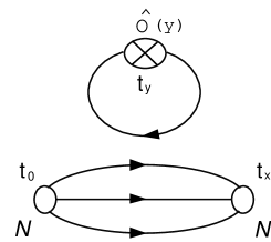
FIG. 3.: Disconnected diagram.

The contribution of the disconnected diagrams represents one of the possible corrections to the nucleon magnetic moment and quark total angular momentum presented in the previous subsection. The disconnected insertion is shown in Fig.3. Disconnected diagrams are difficult to calculate in general because they involve the closed-loop contributions resulting from the self contractions of the quark fields in an observable. An efficient method to obtain the matrix elements is the noise theory discussed in Refs.[36]-[39], explained as follows.

Consider a set of random sources $\eta^{l}(x)$ satisfying

$$\frac{1}{N_{\rm total}}\sum\limits_{l=1}^{N_{\rm total}}\eta^{\dagger l}(x)\eta^{l}(y)=\delta_{xy}\ .$$ (29)

The total number of sources $N_{\rm total}$ is a key parameter controlling the desired statistics. In this work, the random sources $\eta^{l}(x)$ are created by putting $1,~{}-1,~{}i$ or $-i$ randomly on every lattice point for every Dirac and color index. Three-point functions for the disconnected diagrams can now be expressed as:

$$G_{3\alpha\alpha^{\prime}}^{\rm disc}(t_{x},t_{y},{\vec{P}^{\prime}})=G_{2\alpha\alpha^{\prime}}(t_{x},{\vec{P}^{\prime}})\cdot\frac{1}{N_{\rm total}}\sum\limits_{l=1}^{N_{\rm total}}\sum\limits_{{\vec{z},\vec{y}}}\eta^{\dagger l}(y)[{\vec{y}}\times\widehat{O}(y)]M^{-1}(y,z)\eta^{l}(z)\ ,$$ (30)

where $\widehat{O}=\vec{j}^{\rm cons}$ or $T^{j0}$, $G_{2\alpha\alpha^{\prime}}(t_{x},{\vec{P}^{\prime}})$ is Green’s two-point function, and $M^{-1}(y,x)$ is a Wilson-fermion propagator.

Unfortunately, this method requires a large $N_{\rm total}$ to obtain reasonable statistics, which is very expensive in practical simulations. It was discussed in Refs.[38, 39] that the so-called expansion method can expedite the calculation significantly. The idea is to approximate the full fermion propagator,

$$M^{-1}(x,y)=\frac{1}{\delta_{xy}-\kappa P_{xy}}\ ,$$ (31)

where $P_{xy}=\sum\limits_{\mu}[(1+\gamma_{\mu})U_{\mu}(x)\delta_{x,y-\hat{\mu}}+(1-\gamma_{\mu})U^{\dagger}_{\mu}(x-\hat{\mu})\delta_{x,y+\hat{\mu}}]$ by one that includes only the first few terms in the small $\kappa$ expansion,

$$M^{-1}_{\rm exp}(x,y)=\delta_{xy}+\kappa P_{xy}+\kappa^{2}P_{xy}^{2}+...\ .$$ (32)

One then writes $M^{-1}(x,y)=M^{-1}_{\rm exp}(x,y)+\{M^{-1}(x,y)-M^{-1}_{\rm exp}(x,y)\}$. The first term, $M^{-1}_{\rm exp}(x,y)$, can be calculated directly without conjugation gradient, and the remainder, $M^{-1}(x,y)-M^{-1}_{\rm exp}(x,y)$, is computed by the noise method discussed above. Because the remaining contribution is small, the number of random sources needed for the required statistics is considerably reduced.

In this study, we keep ten terms in $M^{-1}_{\rm exp}$. The remainder is calculated with 30 random sources. The results are obtained only for the smallest $\kappa=0.152$ because even in this case the disconnected contribution to the magnetic moment has almost $100\%$ error. For the quark total angular momentum, the result is more stable and the error is about $50\%$. Our final result for the disconnected diagram is $J_{u+d}=-0.12(6)$. This agrees with [17] $J_{u+d}=-0.094(24)$. The negative contribution cancels part of the result from the connected diagram. We have no simple explanation for the sign.

IV Conclusion

In this paper, we report a lattice QCD calculation of the nucleon magnetic moment and the fraction of the nucleon spin carried in the quark total angular momentum. We use the standard Wilson formulation for fermions and 100 quenched configurations in the Monte Carlo evaluations of the Feynman path integrals.

Our results for the magnetic moment cannot be compared directly with the experiment yet. We are uncertain, for example, about the systematic error caused by the quenched approximation, large lattice quark masses, and the finite volume effect. The smallest quark mass in our calculations is about $80~{}{\rm MeV}$ ($\kappa=0.155$) which is about ten times larger than the physical quark mass. The pion mass dependence of the magnetic moment has been studied recently in Refs. [31, 32]. In these papers, a strong dependence on the pion (quark) mass in the region ${m_{\pi}}^{2}<0.5~{}{\rm GeV}$ is suggested. A phenomenological chiral extrapolation of the previous lattice results to the physical pion mass gives results consistent with experimental values.

One interesting finding of this study is that the magnetic form factors, magnetic moment, and the quark total angular momentum decrease with the quark masses. The most plausible explanation is that when the quark mass becomes lighter, the nucleon size grows, and the present lattice volume cannot fully accommodate a physical nucleon.

We have also studied the contribution of the disconnected diagrams to various physical observables. The error bars grow very significant at small quark masses. The sea contribution to the quark total angular momentum is found to be negative. The fraction of the nucleon spin carried by the up and down quark angular momentum is $J_{q}=0.35\pm 10$ at $\kappa=0.152$. The result for a fully dynamical simulation will be reported elsewhere.

- [1] The European Physical Journal C 3, 613 (1998).
- [2] T. Draper, R. M. Woloshyn and K. F. Liu, Phys. Lett. 234, 121 (1990).
- [3] D. B. Leinweber, R. M. Woloshyn and T. Draper, Phys. Rev. D 43, 1659 (1991).
- [4] W. Wilcox, T. Draper and K. F. Liu, Phys. Rev. D 46, 1109 (1992).
- [5] S. Capitani et al., hep-lat/9711007.
- [6] S. J. Dong, K. F. Liu and A. G. Williams, Phys. Rev. D 58, 074504 (1998).
- [7] A. G. Williams., Nucl.Phys.Proc.Suppl. 73, 306 (1999).
- [8] K. F. Liu et al., Phys. Rev. D 49, 4755 (1994).
- [9] J. M. Flynn, ICHEP 96, 335 (1996). See also hep-lat/9611016.
- [10] J. M. Flynn, hep-lat/9710080.
- [11] S. Capitani et al., Nucl.Phys.Proc.Suppl. 73, 294 (1999).
- [12] J. D. Jackson, Classical Electrodynamics (John Wiley & Sons, New York, 1975).
- [13] S. Boffi, C. Giusti and F. D. Pacati, Phys. Rep. 226, 1 (1993); M. Anselmino, A. Efremov and E. Leader, Phys. Rep. 261, 1 (1995); E. W. Hughes and R. Voss, Ann. Rev. Nucl. Part. Sci. 49, 303 (1999); B. Lampe and E. Reya, Phys. Rep. 332, 2 (2000).
- [14] B. W. Filippone and X. Ji, Advances in Nuclear Physics 26, 7 (2001).
- [15] X. Ji, Phys. Rev. Lett. 78, 610 (1997); Phys. Rev. 55, 7114 (1997).
- [16] See for example, X. Ji, J. Phys. G 24, 1181 (1998); A. V. Radyushkin, hep-ph/0101225; K. Goeke, M. V. Polyakov, M. Vaderhaeghen, Prog. Part. Nucl. Phys. 47, 401 (2001).
- [17] N. Mathur et al., Phys. Rev. D 62, 114504 (2000).
- [18] J. D. Bjorkin and S. D. Drell, Relativistic Quantum Mechanics (McGraw-Hill Inc., 1964).
- [19] K. Wilson, Phys. Rev. D 10, 2445 (1974).
- [20] H.J. Rothe, Lattice Gauge Theories (World Scientific, Singapore, 1997).
- [21] A. Pochinsky, Ph.D. thesis (1997).
- [22] R. Gupta et al., Phys. Lett. B 164, 347 (1985).
- [23] J. Ashman et al., Phys. Lett. B 202, 603 (1988).
- [24] D. B. Leinweber, T. Drapper and R. M. Woloshyn, Phys. Rev. D 48, 2230 (1993).
- [25] L. H. Karsten and J. Smit, Nucl. Phys. B 316, 103 (1981).
- [26] G. Martinelli, C. T. Sachrajda, Nucl. Phys. B 316, 355 (1989).
- [27] G. Martinelli, C. T. Sachrajda, Nucl. Phys. B 306, 865 (1988).
- [28] M. C.K. Yang and D. H. Robinson, World Scientific Series in Computer Science 4, 150 (1986).
- [29] Madras, Journal of Stat. Phys. 50, 109 (1988).
- [30] J. Shao and D. Tu, The Jacknife and Bootstrap (Springer Verlag, New York, 1995).
- [31] D. B. Leinweber, D. H. Lu and A. W. Thomas, Phys. Rev. D 60, 034014 (1999).
- [32] D. B. Leinweber, A. W. Thomas and R. D. Young, Phys. Rev. Lett. 86, 5011 (2001).
- [33] J. W. Chen and X. Ji, Phys. Rev. Lett. 87, 152002 (2001); hep-ph/0105197; hep-ph/0111048.
- [34] I. Balitsky and X. Ji, Phys. Rev. Lett 79, 1225 (1997); Phys. Rev. Lett. 76, 740 (1996).
- [35] S. Sasaki, T. Blum, S. Ohta and K. Orginos, hep-lat/0110053.
- [36] C. Thron, S. J. Dong, K. F. Liu and H. P. Ying, Phys. Rev. D 57, 1642 (1997).
- [37] W. Wilcox, Nucl. Phys. Proc. Suppl. 83-84, 834 (2000).
- [38] W. Wilcox, Nucl. Phys. Proc. Suppl. 94, 319 (2001).
- [39] N. Mathur and S.-J. Dong, Nucl. Phys. Proc. Suppl. 94, 311 (2001).