Abstract

Chiral perturbation theory gives direct and unambiguous predictions for the form of various two-point hadronic correlators at low momentum in terms of a finite set of couplings in a chiral Lagrangian. In this paper we study the feasibility of extracting the couplings in the chiral Lagrangian (through 1-loop order) by fitting two-point correlators computed in lattice QCD to the predicted chiral form. The correlators are computed using a pseudofermion technique yielding all-point quark propagators which allows the computation of the full four-momentum transform of the two-point functions to be obtained without sacrificing any of the physical content of the unquenched gauge configurations used. Results are given for an ensemble of dynamical configurations generated using the truncated determinant algorithm on a large coarse lattice. We also present a new analysis of finite volume effects based on a finite volume dimensional regularization scheme which preserves the power-counting rules appropriate for a chiral Lagrangian.

1 Introduction

The introduction of the concept of an effective chiral Lagrangian [1], and the subsequent development of systematic chiral perturbation theory [2], have led to remarkable clarifications in our understanding of the properties of quantum chromodynamics (QCD) in the low-momentum regime. Much of the phenomenology of the interactions of hadrons at low energies can be understood and organized using chiral theory, where the basic degrees of freedom are colorless light hadrons, rather than the quarks and gluons appropriate for a description at (presumably arbitrarily) short distance scales. Of course, the parameters in a chiral effective Lagrangian are ultimately determined by the underlying microscopic theory, i.e. the QCD Lagrangian. The connection between the underlying theory and the chiral Lagrangian is however completely nonperturbative, so any determination of chiral parameters from QCD must have recourse to a systematic nonperturbative calculational procedure: at the present time, this means lattice gauge theory.

Perhaps the most direct and unambiguous predictions of chiral perturbation theory refer to the low-momentum behavior of various two-point correlators of hadronic densities and currents. Typically, the low-momentum expansion of these correlators is ordered in a series of increasing powers of the momentum-squared $p^{2}$, with the power-counting rule $m_{\pi}^{2}\simeq p^{2}$. The leading order term is then determined by the lowest-dimension part ${\cal L}_{2}$ of the full chiral Lagrangian ${\cal L}_{\rm chir}={\cal L}_{2}+{\cal L}_{4}+...$ treated at tree level, the next to leading term at low-momentum in hadronic correlators is obtained from use of ${\cal L}_{2}$ at one-loop level, together with ${\cal L}_{4}$ at tree-level, and so on. In this paper we show that the accurate extraction of up to the leading three terms of this expansion is perfectly feasible by simulation of the relevant correlators in lattice gauge theory. We use exclusively unquenched configurations throughout, so there are no issues of quenched chiral logs, for example. However, the great expense needed to generate decorrelated dynamical configurations at light quark mass (our configurations were generated using the truncated determinant algorithm (TDA) [3]) makes it obviously desirable to extract the maximum possible physical content from each gauge configuration. Consequently, we have used a stochastic pseudofermion technique [4],[5] to obtain all-point quark propagators for each gauge configuration. This means that the Fourier transform used to determine each two-point correlator studied

$$\Delta(p)=\sum_{x,y}e^{ip\cdot(x-y)}<O(x)O(y)>$$ (1)

contains a double sum over all points on the lattice and therefore a factor of the lattice volume more terms than the equivalent correlator studied with single-source or single-sink quark propagators.

Another aspect of calculations performed on discrete space-time lattices is the necessary presence of an infrared (large-distance) cutoff. In this paper we present results for hadronic correlators on a physically large but coarse lattice (6⁴ lattice with lattice spacing $a$=0.4 F, O(a²) improved gauge action) at two different sea-quark masses (note: in all the calculations the valence and sea-quark masses are kept the same). Using a finite volume generalization of dimensional regularization, we have computed the appropriate finite volume modifications of the chiral formulas of Ref.[2]. Of course, the systematic errors induced by lattice discretization will require availabity of a variety of unquenched lattices at differing couplings.

The presentation of our results in this paper is organized as follows. In Section 2, we review the all-point pseudofermion technique [4],[5] used to obtain quark propagators for the measurement of hadronic correlators (for a more detailed study of the statistical features and computational cost of this method see [6]). In Section 3, we present results for the pseudoscalar-pseudoscalar two-point function for our unquenched lattice ensemble. In particular, we show that consistent fits to the predicted chiral form can be obtained, determining the corresponding one-loop chiral Lagrangian parameters to a (statistical) accuracy of a few percent. Moreover, the fitted higher order coefficients are quite small, suggesting that chiral perturbation theory can continue to be accurate for surprisingly high momentum (the chiral fits are extended up to $q^{2}\simeq$2.5 GeV²). In fact, the calculations presented here of higher order chiral coefficients really provide a quantitative nonperturbative basis for estimating the accuracy of low order chiral perturbation theory. In Section 4, we repeat this procedure for the axial vector-axial vector current correlator. Section 5 contains a discussion of the finite volume dimensional regularization technique we have used to derive systematically the finite volume corrections to the chiral formulas for hadronic correlators. Of course other important systematic errors, primarily those due to lattice discretization, can only be addressed once a much larger selection of dynamical lattice ensembles at various lattice spacings and with improved quark actions are available.

2 Computing Hadronic Correlators with All-point Quark Propagators

The dynamical configurations used in the present work represent a very high investment in computational effort. Each new configuration generated using the truncated determinant algorithm [3] requires evaluation of several hundred low eigenvalues of the hermitian Wilson-Dirac (or clover) operator. On a 1.5 GHz Pentium 4 processor, this takes 3 minutes for a 6⁴ lattice and about 80 minutes for a 10³x20 lattice. Decorrelation of physical quantities can take anywhere from 50 to several hundred such updates. The very high cost of generating properly decorrelated unquenched gauge configurations makes it essential to squeeze the maximum physical information content from each available configuration. Conventional quark propagators obtained by (say) a conjugate gradient algorithm only provide the quark propagation amplitude from a single source vector (either point or smeared) to any other point on the lattice: accordingly, the computation of a two-point correlator such as Eq(1) would require fixing either point $x$ or $y$ (typically, at the lattice origin), which obviously sacrifices a great deal of physical information in the gauge configuration. The results presented in this paper will involve correlators computed from all-point quark propagators which give the quark propagation amplitude from any point on the lattice to any other point.

Here we describe briefly an approach (originally suggested by Michael and Peisa in the context of static quark systems, [5]) to obtaining such propagators by simulating bosonic pseudofermion fields. For each quark propagator needed in the hadronic observable of interest (in the case of two-point current correlators, there are two quark propagators which must be multiplied and traced appropriately) introduce a bosonic pseudofermion field $\phi_{ma}$ with action ($m$ a lattice site, $a$ the spin-color index, $Q$ the Wilson or clover operator):

$$S(\phi) = \phi^{\dagger}Q^{\dagger}Q\phi$$ (2)

$$= \phi^{\dagger}H^{2}\phi,\;\;\;H\equiv\gamma_{5}Q=H^{\dagger}$$ (3)

For a given fixed background gauge field $A$, simulating the pseudofermion field with the preceding action produces the following correlator ($<<O>>$ means the average of $O$ relative to the measure $e^{-S}$) :

$$<<\phi_{ma}\phi^{*}_{nb}>>_{S(\phi)} = (H^{-2})_{ma,nb}$$ (4)

$$<<\phi_{ma}(\phi^{\dagger}H)_{nb}>>_{S(\phi)} = (H^{-1})_{ma,nb}$$ (5)

$$= (Q^{-1}\gamma_{5})_{ma,nb}$$ (6)

Note that separate pseudofermion fields are needed for each quark propagator as averages of four-point bosonic pseudofermion amplitudes will produce contractions with the wrong sign relative to the corresponding fermionic 4 quark amplitudes. However, it turns out that the computational effort required is quite manageable, allowing us to obtain sufficiently accurate all-point propagators with only a few times the computer time required for a conventional conjugate-gradient evaluation of the corresponding single-source propagator. The reasons for this are twofold:
(i) The pseudofermion average $<<....>>$ is efficiently implemented by a heat-bath update of pseudofermion fields. As the pseudofermion action is a Gaussian one, the statistical properties of this simulation are essentially trivial (gauge configuration updates, by contrast, involve an action with a highly nonlinear dependence on the field degrees of freedom), and contain no surprises.
(ii) For a fixed gauge field, most quantities decorrelate after a few pseudofermion sweeps. For low-momentum quantities, the presence of low eigenmodes of the hermitian Wilson operator $H$ can lead to long autocorrelations, but these can be handled by projecting out the corresponding low modes, which reduces the condition number and restores a more rapid decorrelation (see [6]). However, even without such projections, we are able to obtain the momentum dependence of the correlators sufficiently accurately to allow good fits to the chiral behavior.

It is easy to see that the computation of multipoint hadronic correlators involving $n$ quark propagators can be reduced to convolutions of $n$ pseudofermion fields, rapidly computed by fast Fourier transform (FFT). (This is so both for local and smeared hadronic operators, although the quantities studied in this paper are exclusively local densities and currents.) For example, the full 4-momentum transform $\Delta(q^{2})\equiv\sum_{x,y}e^{iq\cdot(x-y)}\Delta(x,y)$ of the 2-point pseudoscalar correlator is given by

$$\Delta(x,y) = <0|T\{\bar{\Psi}(x)\gamma_{5}\Psi(x)\;\bar{\Psi}(y)\gamma_{5}\Psi(y)\}|0>$$ (7)

$$= -<\rm{tr}((Q^{-1}\gamma_{5})_{xy}(Q^{-1}\gamma_{5})_{yx})>$$

$$= -<<\sum_{ab}\phi_{xa}(\phi^{\dagger}H)_{yb}\chi_{yb}(\chi^{\dagger}H)_{xa}>>$$

$$= -<<(\phi^{\dagger}H\chi)_{yy}(\chi^{\dagger}H\phi)_{xx}>>$$

which becomes an easily evaluated fast Fourier transform of products of pseudofermion fields:

$$\Delta(q^{2})=-<<\rm{FFT}(\chi^{\dagger}H\phi)(q)\rm{FFT}(\phi^{\dagger}H\chi)(-q)>>$$ (8)

Our main purpose in this paper is to show that the chiral behavior of QCD hadronic correlators can be studied directly in momentum space and higher order chiral couplings extracted with high statistical accuracy. The unquenched lattices used here lattices are a large ensemble (800 configurations) of physically large, coarse lattices recently used in a study of stringbreaking [7] (lattice spacing 0.4 Fermi, but with O($a^{2}$) improvement of the gauge action [8]: thus, the gauge action includes the usual plaquette term as well as a twisted rectangle (“trt”) operator), and at a sea-quark kappa value of 0.2050. Quark eigenmodes up to 420 MeV are included exactly in the determinant. In this lattice ensemble, the determinant contribution to the measure corresponds to two degenerate light quark flavors (corresponding to $M_{\pi}\simeq$200 MeV, where the lattice scale is fixed from stringtension measurements).

We conclude this section by describing the computational effort required for evaluation of the pseudofermion average (7) on a single gauge configuration. For the 6⁴ lattices, a single heat-bath update of the two pseudofermion fields $\phi,\chi$ requires 0.366 sec. on a 1.5 GHz Pentium-4 processor. The convolutions and FFT operations required to obtain the desired four-momentum field $\Delta(q^{2})$ in (8) require an additional 0.024 sec. and are performed after every 2 heat-bath updates of $\phi,\chi$. The final pseudofermion average for $\Delta(q^{2})$ was obtained from 20000 measurements, corresponding to 2.1 Pentium-4 hrs.

3 Extracting Chiral Parameters from Pseudoscalar Correlators

Among the most basic predictions of chiral perturbation theory are expressions for the low momentum behavior of correlators of hadronic densities and currents, first derived by Gasser and Leutwyler [2]. In this section we study the extent to which a lattice computation of the two-point function of the isovector pseudoscalar density $\bar{\psi}\tau_{i}\gamma_{5}\psi$ (here, $\tau_{i}$ are the isospin generators for SU(2), $\psi$ the isodoublet quark field) can be used to constrain the parameters of the chiral effective Lagrangian. We work throughout with two flavors of degenerate light dynamical quarks, so the relevant chiral group is SU(2)xSU(2), and we will adhere as much as possible to the notation of Ref [2], the results of which are in any event restricted to exactly this two-flavor case.

Defining $\tau_{\pm}\equiv\frac{1}{2}(\tau_{1}\pm i\tau_{2})$, the correlator computed in (7-8) corresponds to

$$\Delta_{PS-PS}(q^{2})=\int d^{4}x<\bar{\psi}\tau_{-}\gamma_{5}\psi(x)\bar{\psi}\tau_{+}\gamma_{5}\psi(y)>e^{iq\cdot(x-y)}$$ (9)

with the low-momentum chiral behavior (in infinite volume Euclidean space) [2]:

$$\Delta_{PS-PS}(q^{2})\simeq\frac{1}{2}(\frac{G_{\pi}^{2}}{q^{2}+M_{\pi}^{2}}+\frac{B^{2}}{2\pi^{2}}(l_{4}-h_{1})+O(q^{2}))$$ (10)

and with the pseudoscalar decay constant $G_{\pi}$ defined as

$$G_{\pi}\delta_{ij}\equiv<0|\bar{\psi}\tau_{i}\gamma_{5}\psi|\pi_{j}>$$ (11)

The quark condensate $<0|\bar{\psi}_{i}\psi_{j}|0>=F_{\pi}^{2}B\delta_{ij}$ fixes the constant $B$, and $l_{4},h_{1}$ are couplings in the O($p^{4}$) chiral Lagrangian. Our object here is to determine the latter as accurately as possible using lattice data. The fits will also provide information on the size of even higher order terms (e.g. O($p^{2}$) in the pseudoscalar correlator), which is clearly relevant to the issue of accuracy of chiral perturbation theory through one loop order.

We begin by describing the results obtained from our ensemble of 800 6⁴ lattices. These large coarse lattice configurations are O(a²) improved with respect to the gauge action, but the quark action is unimproved Wilson, so the results obtained will necessarily contain large systematic effects (relative to the corresponding continuum parameters), although we shall see that the statistical errors are extremely small. The configurations were generated using the TDA algorithm [3] to include virtual quark-loop effects of a doublet of degenerate light sea quarks exactly up to a quark off-shellness of about 420 MeV. The average value obtained for $\Delta_{PS-PS}(q^{2})$ for this ensemble is shown in Fig.1. For nonzero momentum, the statistical errors are smaller than the symbol size. The range of $q^{2}$ corresponds to lattice values from 0 to 16, with a unit of $q^{2}$ on the lattice corresponding to 0.25 GeV² in physical units. The comparatively large error at the zero momentum point is attributable to the autocorrelations induced by low eigenmodes of $H$ (see [6] for a solution of this problem). In fact, our results for the nonzero momentum modes are sufficiently accurate that we will discard the zero-momentum point entirely in performing the fits to Eq(10).

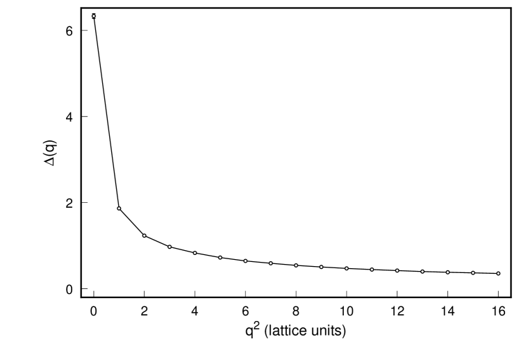
Figure 1: Measured pseudoscalar correlator (ensemble of 800 6⁴ lattices) $\Delta(q^{2})$

Table 1: Dependence of fitted pion mass on momentum fitting range.

$q^{2}{\rm range}$	$M_{\pi}$	$\chi^{2}/{\rm d.o.f}$
1-8	0.324$\pm$ 0.033	3.6
1-9	0.352$\pm$ 0.026	2.7
1-10	0.422$\pm$ 0.020	2.6
1-11	0.449$\pm$ 0.017	2.3
1-12	0.480$\pm$ 0.015	2.2
1-13	0.530$\pm$ 0.013	2.7

As the pseudoscalar correlator (9) involves by definition only local operators, it may be wondered whether there is much hope of extracting an accurate pion mass $M_{\pi}$ in (10). The excited state contamination which would normally require the use of smeared sources/sinks to obtain an accurate pion mass appears as contributions to the higher order chiral contributions (of order O($q^{0},q^{2},q^{4}$…)). A conventional cosh fit to 800 smeared-local correlators at $\kappa=$0.2050 gives an alternative determination of the pion mass for this ensemble: $M_{\pi}=0.396\pm 0.007$ (or about 200 MeV in physical units, with the scale determined from string tension measurements [7]: the use of an unimproved Wilson action on this coarse a lattice makes spin-dependent scales such as the rho unreliable). The inevitable breakdown of chiral perturbation theory in the ultraviolet means that we cannot expect the fit to give meaningful results if the momentum range is too large. Indeed, we find that, allowing the pion mass to vary freely in a fit of the form

$$\Delta(q^{2})=\frac{A_{1}}{q^{2}+M_{\pi}^{2}}+A_{2}+A_{3}q^{2}+A_{4}(q^{2})^{2}$$ (12)

the fit values for $M_{\pi}$ increase well beyond the physical value if the fit range is extended beyond $q^{2}\simeq$2.5 GeV² (see Table 1). There is a broad minimum in the chisquared per degree of freedom for the momentum range $1\leq q^{2}\leq 10-12$: choosing the UV cutoff in our fits at $q^{2}=10$ (lattice units,$\simeq 2.5$Gev²) gives a fitted pion mass very close to the value found using smeared source correlators.

Figure 2: Fit of measured pseudoscalar correlator $\Delta(q^{2})$, $1\leq q^{2}\leq 10$

A five parameter fit of the formula (12) performed on the range $1<q^{2}<10$ yields (see Fig. 2) the following results:

$$A_{1} = 1.52\pm 0.029$$

$$M_{\pi} = 0.422\pm 0.020$$

$$A_{2} = 0.622\pm 0.010$$

$$A_{3} = -0.0460\pm 0.0015$$

$$A_{4} = 0.00163\pm 0.00007$$ (13)

with a $\chi^{2}/{\rm d.o.f}=2.6$. The pion mass is consistent within errors with the value quoted above, determined from a study of smeared-local correlators. The remarkable statistical accuracy of this method is apparent in the errors for the leading order residue $A_{1}$ and the one-loop chiral parameter $A_{2}$, both of which are determined at the 2% level for the statistical error! Moreover, the higher order coefficients ($O(q^{2},q^{4})$ terms) are very small, which bodes well for the accuracy of chiral perturbation theory through one-loop, even at quite high momenta. Repeating the fit with the pion mass held fixed at the value $M_{\pi}=$0.396 determined from fits of smeared-local correlators gives a somewhat improved $\chi^{2}/{\rm d.o.f}$=2.2, with the fitted parameters statistically indistinguishable from the results in (13). However, removing the $q^{4}$ term in (12) results in fits with much higher $\chi^{2}/{\rm d.o.f.}>$5, and fit parameters $A_{1},A_{2}$ and $M_{\pi}$ differing substantially from the values obtained in (13) if the momentum range is extended beyond $q^{2}=$6, corresponding to 1.5 GeV² in physical units. The value of the pion decay constant will be obtained from a study of the axial-vector correlator in the next section: we find $F_{\pi}=$0.187$\pm$0.011. The critical kappa value is most readily extracted from the predicted topological charge distributions of Leutwyler and Smilga [9],[10]: one finds $\kappa_{c}$=0.2067, corresponding to a bare quark mass for $\kappa=0.2050$ of $\hat{m}=$0.020. On the other hand, using the value for $F_{\pi}$ quoted above, the bare quark mass can be extracted from the chiral Ward identity

$$\hat{m}=\frac{F_{\pi}M_{\pi}^{2}}{G_{\pi}}$$ (14)

where from (10,13) we find $G_{\pi}=$1.74$\pm$0.02. Accordingly (taking $M_{\pi}=$0.422), (14) yields a bare quark mass

$$\hat{m}=0.0191\pm 0.0021$$ (15)

consistent with the $\kappa_{c}$ value extracted from the topological analysis.

4 Extracting Chiral Parameters from Axial Current Correlators

In this section we shall describe our results for the nonperturbative lattice evaluation of the axial vector correlator, using the same lattice ensemble described in the preceding section. Defining

$$\Delta_{AX-AX}^{\mu\nu}(q)=\int d^{4}x<\bar{\psi}\tau_{-}\gamma_{5}\gamma^{\mu}\psi(x)\bar{\psi}\tau_{+}\gamma_{5}\gamma^{\nu}\psi(y)>e^{iq\cdot(x-y)}$$ (16)

we have used the pseudofermion technique to extract the contracted scalar quantity (in Euclidean space)

$$\Delta_{AX-AX}(q^{2})\equiv\frac{1}{2}g_{\mu\nu}\Delta_{AX-AX}^{\mu\nu}(q)$$ (17)

The prediction of chiral perturbation theory for this contracted axial-vector correlator can be summarized in the formula [2] :

$$\Delta_{AX-AX}(q^{2})\simeq\frac{F_{\pi}^{2}q^{2}}{q^{2}+M_{\pi}^{2}}-4F_{\pi}^{2}+\frac{1}{16\pi^{2}}(l_{5}-h_{2})q^{2}+O(q^{4})$$ (18)

where the term involving $l_{5}-h_{2}$ represents a contribution from the O($p^{4}$) chiral Lagrangian. The constant term $-4F_{\pi}^{2}$ in (18) arises from a contact term $\propto\delta^{4}(x-y)$ in the coordinate space correlator which is highly UV-divergent and not accessible from our lattice calculation, so we have allowed this constant to float freely in our fits.

Figure 3: Measured axial-vector correlator $\Delta_{ax-ax}(q^{2})$, fit $0\leq q^{2}\leq 10$

We have computed $\Delta_{AX-AX}(q^{2})$ using the pseudofermion approach: for the ensemble of 800 lattice configurations, the results are shown in Fig. 3. Again, the statistical errors are quite small. With the fitting formula

$$\Delta_{AX-AX}(q^{2})=\frac{F_{\pi}^{2}q^{2}}{q^{2}+M_{\pi}^{2}}+A_{1}+A_{2}q^{2}+A_{3}q^{4}$$ (19)

a conservative fit using only the $q^{2}$ range from 0 to 4 (lattice units) and setting the higher order $A_{3}$ term to zero, one finds $F_{\pi}=$0.213$\pm$0.010 with a $\chi^{2}/{\rm dof}$ of 0.8/2. In this fit we have fixed the pion mass at the value 0.422 determined in the preceding section from the pseudoscalar correlator fits. The higher order coefficients are determined as $A_{1}=$0.8157$\pm$0.0040, $A_{2}=$0.0602$\pm$0.0004 respectively. The statistical error on these higher order chiral coefficients is again very small, indicating the high statistical content available in an all-point approach. The contact term $A_{1}$ is stable to three significant figures with respect to changing the fitting range to $0\leq q^{2}\leq$3 or $0\leq q^{2}\leq$5, as it is completely dominated by ultraviolet contributions (see discussion above). Another point worth noting here is that our momentum-space approach allows the extraction of meaningful chiral parameters at light quark mass from a local-local axial-vector correlator, something which would be impossible using conventional Euclidean coordinate space fits.

Keeping only terms up to order $q^{2}$ in the chiral fitting formula, one finds in the case of the axial-axial correlator that the chisquared deteriorates much more rapidly as higher momenta are included in the fitting range than in the case of the pseudoscalar correlators discussed in the preceding section. If a $q^{4}$ term is included in the fit, then the fitting range can be extended considerably. In Fig. 3 the chiral fit obtained for a fitting range $0\leq q^{2}\leq$10 is shown: the $\chi^{2}/{\rm dof}$ for this fit is 14/7. The extracted chiral parameters in this case are:

$$F_{\pi} = 0.187\pm 0.011$$

$$A_{1} = 0.8148\pm 0.0038$$

$$A_{2} = 0.0777\pm 0.0003$$

$$A_{3} = -0.00442\pm 0.00002$$ (20)

5 Finite Volume Effects

5.1 Dimensional Regularization at Finite Volume

In order to reliably extract the parameters of the chiral Lagrangian out of equations (12) and (19) and the values in equation (13) and (20), we need a generalization of equations (10) and (18) that includes finite volume effects. At the same time this generalization should preserve the power counting rules appropriate for chiral perturbation theory. Here we present such a generalization by extending the dimensional regularization scheme to finite volume with periodic boundary conditions. We assume our system lives in a ${\mathcal{L}}^{4}$ box with the momentum $k_{\mu}$ taking values $\frac{2\pi}{{\mathcal{L}}}n_{\mu}$ where $n_{\mu}$ is an integer.

We start by converting massive propagators to exponential form using Schwinger parameters:

$$\frac{1}{k^{2}+m^{2}}=\int_{0}^{\infty}d\lambda e^{-\lambda(k^{2}+m^{2})}$$ (21)

and replacing the infinite volume loop integrals over $k$ (where $k$ is a d-dimensional vector) by finite sums

$$\mu^{4-d}\int\frac{d^{d}k}{(2\pi)^{d}}f(k_{\mu})\rightarrow\frac{\mu^{4-d}}{(2\pi)^{d}}(\frac{2\pi}{{{\mathcal{L}}}})^{d}\sum_{n_{\mu}}f(\frac{2\pi}{{\mathcal{L}}}n_{\mu})$$ (22)

Once the k-dependence is exponentiated as in (21), we will need to evaluate sums like

$$\sum_{n_{\mu}=-\infty}^{+\infty}e^{-\lambda(\frac{2\pi n_{\mu}}{{\mathcal{L}}})^{2}}\equiv\sqrt{\pi}{\mathcal{I}}(\frac{4\pi^{2}}{{\mathcal{L}}^{2}}\lambda)$$ (23)

so that (22) will involve ${\mathcal{I}}^{d}$, where ${\mathcal{I}}$ is the function

$${\mathcal{I}}(\lambda)\equiv\frac{1}{\sqrt{\pi}}\sum_{n=-\infty}^{+\infty}e^{-\lambda n^{2}}$$ (24)

We will also need to evaluate a generalization of ${\mathcal{I}}(\lambda)$:

$${\mathcal{J}}(\lambda,\beta)\equiv\frac{1}{\sqrt{\pi}}\sum_{n=-\infty}^{+\infty}e^{-\lambda(n^{2}-\beta n)}$$ (25)

where we shall need both ${\mathcal{I}}$ and ${\mathcal{J}}$ in the physically interesting limit $\lambda\rightarrow 0$ corresponding to large but finite volume.

Using the Poisson sum formula one can easily write equations (24) and (25) in a form useful to take that limit:

$${\mathcal{I}}(\lambda)=\frac{1}{\sqrt{\lambda}}\sum_{m=-\infty}^{+\infty}e^{-\frac{\pi^{2}m^{2}}{\lambda}}\simeq\frac{1}{\sqrt{\lambda}}(1+2e^{-\frac{\pi^{2}}{\lambda}}+...)$$ (26)

and

$${\mathcal{J}}(\lambda,\beta)=\frac{1}{\sqrt{\lambda}}e^{\frac{\beta^{2}\lambda}{4}}\sum_{m=-\infty}^{+\infty}e^{-\frac{\pi^{2}m^{2}}{\lambda}}\cos(\pi\beta m)$$ (27)

These equations are all we need to develop the generalization of dimensional regularization to finite volume that preserves the power counting rules appropriate for chiral perturbation theory.

Consider for example the quadratically divergent integral

$$S_{2}\equiv\mu^{4-d}\int\frac{d^{d}k}{(2\pi)^{d}}\frac{1}{k^{2}+m^{2}}$$ (28)

where we work at finite volume. Using the procedure outlined above and changing variables we get

$$S_{2}\equiv\frac{1}{4}\mu^{4-d}\pi^{\frac{d}{2}-2}{\mathcal{L}}^{2-d}\int_{0}^{\infty}d\lambda e^{-\frac{m^{2}{\mathcal{L}}^{2}}{4\pi^{2}}\lambda}{\mathcal{I}}^{d}(\lambda)$$ (29)

Replacing the expression (26) for ${\mathcal{I}}$ we can easily check that the first term in the expansion is identically equal to the infinite volume integral while the other terms correspond to ultraviolet finite exponentially small finite volume corrections. The divergence as $d\rightarrow 4$ is therefore equal to the infinite volume divergence and the $MS$ or $\overline{MS}$ prescriptions remain unmodified.

If $m\mathcal{L}$ in the exponent above is large, the next to leading term in the expansion of ${\mathcal{I}}^{4}$ approximates well the finite volume correction of $S_{2}$. We can make $d=4$ since the term is finite, getting

$$S_{2}^{\mathrm{next\,to\,leading}}=\frac{2}{{\mathcal{L}}^{2}}\int_{0}^{\infty}d\lambda\frac{e^{-\frac{m^{2}{\mathcal{L}}^{2}}{4\pi^{2}}\lambda-\frac{\pi^{2}}{\lambda}}}{\lambda^{2}}=\frac{2}{\pi^{2}}\frac{m}{{\mathcal{L}}}K_{1}(m{\mathcal{L}})$$ (30)

where $K_{1}(x)$ is a modified Bessel function. This is exponentially small when $m{\mathcal{L}}$ gets large. Further corrections fall exponentially at an even faster rate. For the lattice ensemble studied previously, $m{\mathcal{L}}{\sim}2.5$ so this approximation is inadequate and (29) must be evaluated more carefully (see below).

As another example of the finite volume dimensional regularization procedure consider the relation

$$S_{4}\equiv\mu^{4-d}\int\frac{d^{d}k}{(2\pi)^{d}}=0$$ (31)

for the quartically divergent integral. For infinite volume this is the only consistent definition, as there is no available dimensionful quantity other than $\mu$, which can only appear logarithmically in the finite volume part at $d=4$. At finite volume this argument does not work because we have now a new scale ${\mathcal{L}}$. However, as we show next, the relation is also valid at finite volume.

Writing $1$ in the “integrand” as $(m^{2}+k^{2})/(m^{2}+k^{2})$ and introducing again the Schwinger parameter we can easily transform $S_{4}$ into

$$S_{4}=\frac{\mu^{4-d}\pi^{d/2}}{{\mathcal{L}}^{d}}\int_{0}^{\infty}d\lambda e^{-x\lambda}(x-\frac{\partial}{\partial\lambda}){\mathcal{I}}^{d}(\lambda)$$ (32)

where $x=\frac{m^{2}{\mathcal{L}}^{2}}{4\pi^{2}}$ as usual. Separating ${\mathcal{I}}^{d}(\lambda)$ into $\lambda^{d/2}$ and ${\mathcal{I}}^{d}(\lambda)-\lambda^{d/2}$ and replacing each part into the above equation, we get for the first part

$$S_{4}^{\mathrm{divergent}}=\frac{\mu^{4-d}\pi^{d/2}}{{\mathcal{L}}^{d}}\int_{0}^{\infty}d\lambda e^{-x\lambda}(x-\frac{\partial}{\partial\lambda})\lambda^{d/2}$$ (33)

which is identical to the infinite volume version of $S_{4}$ and therefore it must be zero by the standard argument. In fact, analytically continuing equation (33) to $d<0$ and integrating by parts one can see that it is zero as it must be.

The non trivial result is that the finite volume correction

$$S_{4}^{\mathrm{convergent}}=\frac{\mu^{4-d}\pi^{d/2}}{{\mathcal{L}}^{d}}\int_{0}^{\infty}d\lambda e^{-x\lambda}(x-\frac{\partial}{\partial\lambda})({\mathcal{I}}^{d}(\lambda)-\lambda^{d/2})$$ (34)

is also explicitly zero for any $d$, as one can see by replacing the expansion (26) for ${\mathcal{I}}(\lambda)$ above and integrating by parts.

It is now clear that with the procedure outlined in equations (21) to (27) we can compute the finite volume effects in the dimensional regularization scheme. In the next subsection we shall employ this technology to compute the finite volume corrections to the two-point hadronic correlators. This will allow us to estimate quantitatively the systematic errors in the results of Sections 3,4 due to finite size.

5.2 Finite Volume Corrections to Two-Point Hadronic Correlators

Let us find finite volume corrections to the pseudoscalar correlator and the axial vector correlators using the dimensional techniques described above. First, we note that the finite-volume dependence of correlators calculated through O($p^{4}$) in chiral perturbation theory arises from the one-loop integrals using the lowest order chiral Lagrangian for the chiral vertices (see Ref [11]). Since one-loop graphs come from ${\cal L}_{2}$, the evaluation of pseudoscalar and axial vector correlators involves loop integrals of only the type (28) [2]. So in calculating the finite volume corrections to $G_{\pi}$, $M_{\pi}$, and $F_{\pi}$ to one loop order we can simply add the finite correction to this loop integral to the mass logarithm terms in those constants obtained in Ref [2].

The $G_{\pi}$, $M_{\pi}$, and $F_{\pi}$ modifications are then given by

$$G_{\pi}\rightarrow G_{\pi}^{{\mathrm{inf.}}\,{\mathrm{vol.}}}-\frac{B}{F}S_{2}^{F}$$ (35)

$$M_{\pi}\rightarrow(M_{\pi}^{{\mathrm{inf.}}\,{\mathrm{vol.}}})+\frac{M}{4F^{2}}S_{2}^{F}$$ (36)

and

$$F_{\pi}\rightarrow F_{\pi}^{{\mathrm{inf.}}\,{\mathrm{vol.}}}-\frac{1}{F}S_{2}^{F}$$ (37)

where

$$S_{2}^{F}\equiv\frac{1}{4}\frac{1}{{\mathcal{L}}^{2}}\int_{0}^{\infty}d\lambda e^{-\frac{M^{2}{\mathcal{L}}^{2}}{4\pi^{2}}\lambda}({\mathcal{I}}^{4}(\lambda)-\frac{1}{\lambda^{2}})$$ (38)

which corresponds to the finite volume part of $S_{2}$ of equation (29). Since the coefficient in the exponent in the integrand, $M^{2}{\mathcal{L}}^{2}/4\pi^{2}$, is small($\simeq$ 0.16), the contribution from large $\lambda$ is substantial. So the original form (24) for $\mathcal{I}(\lambda)$ is used. The numerical integration using Mathematica yields $S_{2}^{F}$=0.002200. To find the finite volume corrections to the leading order, the values of the constants $F_{\pi}$=0.187$\pm$0.011, and $M_{\pi}$=0.422$\pm$0.020 found in the previous sections are used for $F$, and $M$. With $S_{2}^{F}$ above, the finite volume correction to $M_{\pi}$ is 0.007 and $F_{\pi}$ -0.012. In the finite volume term of $G_{\pi}$there is a constant B(practically, the quark condensate) which was not extracted directly from the previous fits. To the leading order $G_{\pi}=2BF$ [2]. Thus the finite volume correction to $G_{\pi}$ becomes $-G_{\pi}{S_{2}^{F}}/2F_{\pi}^{2}$ to this order. Using a central value of $G_{\pi}$=1.74, we find -0.05 for the finite volume correction to $G_{\pi}$. We see that in all cases the finite volume corrections are on the order of a few percent even for the fairly light quark mass ($M_{\pi}\simeq$ 200 MeV) used in the dynamical lattices studied in Sections 3,4. Of course, these lattices were physically large (2.4 F⁴): on smaller lattices for light quark masses, the finite volume corrections will be more important.

6 Acknowledgements

The work of A. Duncan and J. Yoo was supported in part by NSF grant PHY00-88946.

References

- [1] S. Weinberg, Phys. Rev. 166 (1968) 1568; S. Coleman, J. Wess and B. Zumino, Phys. Rev. 177 (1969) 2239.
- [2] J. Gasser and H. Leutwyler, Ann. Phys. (N.Y.) 158 (1984) 142.
- [3] A. Duncan, E. Eichten and H. Thacker, Phys. Rev. D59 (1998) 014505.
- [4] A. Duncan, E. Eichten and J. Yoo, “Hadronic Correlators from All-point Quark Propagators”, (talk of A. Duncan at Lattice 2001, Berlin, Germany, Aug. 2001).
- [5] C. Michael and J. Peisa, Phys. Rev. D58 (1998) 034506.
- [6] A. Duncan and E. Eichten, “Improved Pseudofermion Approach for All-Point Propagators”, hep-lat/0112028.
- [7] A. Duncan, E. Eichten and H. Thacker, Phys. Rev. D63 (2001) 111501.
- [8] M. Alford, W. Dimm, G.P. Lepage, G. Hockney and P.B. Mackenzie, Phys. Lett. B361 (1995) 87.
- [9] H. Leutwyler and A. Smilga, Phys. Rev. D 46(1992)5607.
- [10] Talk of E. Eichten, Lattice2001, Berlin, Germany Aug. 19-24,2001.
- [11] J. Gasser and H. Leutwyler, Nucl. Phys. B307(1988) 763.