Effective Monopole Action at Finite Temperature in SU(2) Gluodynamics

Abstract:

Effective monopole action at finite temperature in SU(2) gluodynamics is studied on anisotropic lattices. Using an inverse Monte-Carlo method and the blockspin transformation for space directions, we determine 4-dimensional effective monopole action at finite temperature. We get an almost perfect action in the continuum limit under the assumption that the action is composed of two-point interactions alone. It depends on a physical scale $b_{s}$ and the temperature $T$. The temperature-dependence appears with respect to the spacelike monopole couplings in the deconfinement phase, whereas the timelike monopole couplings do not show any appreciable temperature-dependence. The dimensional reduction of the 4-dimensional SU(2) gluodynamics ((SU(2))_4D) at high temperature is the 3-dimensional Georgi-Glashow model ($(GG)_{3D}$). The latter is studied at the parameter region obtained from the dimensional reduction. We compare the effective instanton action of $(GG)_{3D}$ with the timelike monopole action obtained from (SU(2))_4D. We find that both agree very well for $T\geq 2.4T_{c}$ at large $b$ region. The dimensional reduction works well also for the effective action.

1 Introduction

It is important to understand nonperturbative effects of Quantum Chromodynamics (QCD) at finite temperature. At zero temperature, the typical nonperturbative phenomena are color confinement and the chiral symmetry breaking. At high temperature, QCD enters the Quark Gluon Plasma (QGP) phase in which colors are deconfined and chiral symmetry is restored. It is known that not only perturbative but also nonperturbative effects such as the spatial string tension and the Debye-screening mass [1] exist even in the deconfinement phase.

The nonperturbative quantities have been studied also using the 3-dimensional effective action obtained through the dimensional reduction. The idea of the dimensional reduction for high temperature gauge theory was proposed in early 80’s [2]. The 3-dimensional effective action is derived perturbatively by the integration of non-zero modes for time direction of the fields. After performing the dimensional reduction perturbatively in (SU(2))_4D, the obtained effective action is $(GG)_{3D}$. The effectiveness of the dimensional reduction at high temperature has been confirmed by numerical simulations on the lattice [1,3–7]. Quadratic and quartic interactions of the Higgs field are necessary for the infrared physics. Spacelike Wilson loops and Polyakov loop correlators in $(GG)_{3D}$ agree well with those of (SU(2))_4D for $T\geq 2T_{c}$ [3]. The details of the relation between the phase diagram and the parameter region of the dimensional reduced $(GG)_{3D}$ in 2-loop perturbative calculation have been studied in  [5]. Using the parameter in 2-loop perturbative calculation, the Debye-screening mass is shown to be a nonperturbative physical quantity in itself [1]. The validity of the dimensional reduction for $T\geq 2T_{c}$ in (SU(2))_4D have also been confirmed for the glueball spectrum [6] and the gauge-fixed propagator [7]. In Ref. [8] the parameters of the dimensional reduced effective action have been determined nonperturbatively. However to the authors’ knowledge, there have been no nonperturbative studies using the dimensional reduction from the standpoint of topological quantity.

Figure 1: Physical string tensions (circle) and spatial string tensions (square) from monopoles in SU(2)QCD on $24^{3}\times 8$ lattices. This figure is from Ref. [13].

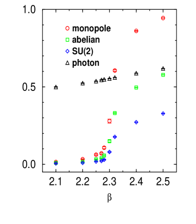
Figure 2: Non-abelian and abelian Polyakov loops and monopole Dirac string and photon contributions to Polyakov loops in the MA gauge in SU(2) QCD on $24^{3}\times 4$ lattice. This figure is taken from Ref. [16].

At zero temperature, the dual superconductor picture of the QCD vacuum seems to be the color confinement mechanism in which magnetic monopoles condense and color-electric flux is squeezed (dual Meissner effect). Monopoles are induced by performing abelian projection (partial gauge-fixing keeping $U(1)^{2}$). In SU(2) and SU(3) gauge theory, the string tension extracted from the monopole part reproduces the original one (monopole dominance). This fact suggests that monopoles play an important role for confinement. An effective monopole action described by monopole currents has been studied in detail and an almost perfect action (corresponding to the continuum limit) is derived successfully in infrared region of QCD [9–11].

At finite temperature, there have been interesting data suggesting the importance of monopoles [12–16]. The string tension from the monopole part of the Wilson loop almost agrees with that of the abelian Wilson loop in the confinement phase, whereas it vanishes clearly in the deconfinement phase. The data [13] for the temperature-dependence of the string tensions from monopoles and photons are shown in Fig. 2. The string tension from the photon part is negligibly small.

A non-abelian Polyakov loop is well known as an order parameter of the deconfinement phase transition. Similarly an abelian Polyakov loop which is written in terms of abelian link variables alone is an order parameter of the deconfinement phase transition. It is given by a product of contributions from Dirac strings of monopoles and from photons. The data [16] of SU(2) QCD in the MA gauge are shown in Fig. 2. Here the confinement-deconfinement phase transition occurs at the critical coupling $\beta_{c}=2.298$. The abelian Polyakov loops vanish in the confinement phase whereas they have a finite value in the deconfinement phase. The behaviors of the Dirac string contributions (monopole Polyakov loops) are similar, but more drastic than those of the abelian and the non-abelian Polyakov loops. The photon part has a finite non-zero value in both phases. So only the monopole Polyakov loops play a role as an order parameter of the deconfinement phase transition in the abelian Polyakov loops.

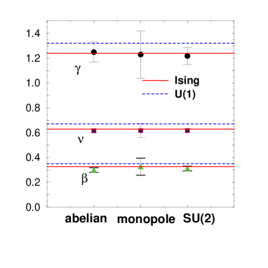
Figure 3: Critical exponents of non-abelian, abelian and monopole Polyakov loops in SU(2) QCD. This figure is taken from Ref. [16].

The critical exponents have been determined from the behaviors of the Polyakov loops, their susceptibility and the fourth cumulant. The data [16] are shown in Fig. 3. The critical exponents and the critical temperature determined in the abelian and the monopole case are in agreement with those in the non-abelian case within the statistical error.

What happens with respect to the nonperturbative effects at high temperature ? There is also the monopole dominance for spatial string tension at high temperature  [13]. It is known that the timelike wrapped monopole loops are important which are closed through the periodic boundary condition [17]. On the other hand, $(GG)_{3D}$ has an instanton solution  [18, 19] and its Coulomb gas leads us to confinement [20, 21]. 4D timelike monopoles tend to instantons in the high temperature limit. These facts suggest that at high temperature nonperturbative effects are caused by timelike monopoles (when $T\geq T_{c}$) and instantons (when $T\to\infty$).

It is the purpose of this paper to confirm the above expectation. We derive first infrared effective monopole actions numerically from finite temperature (SU(2))_4D . We adopt anisotropic lattices and perform the blockspin transformations of the monopole currents to study the continuum limit. The behaviors of spacelike monopole action and timelike monopole action in the confinement and in the deconfinement phases are discussed carefully. We then compare the timelike monopole effective action at high temperature in (SU(2))_4D with the effective instanton action derived numerically from $(GG)_{3D}$ to study if the dimensional reduction works also in the framework of effective monopole (instanton) action.

The paper is organized as follows. In Section 2 we consider the effective monopole action at finite temperature in (SU(2))_4D on anisotropic lattices. In Section 3 we investigate the instanton action in $(GG)_{3D}$ and compare it with the timelike monopole action in (SU(2))_4D at high temperature. Section 4 is devoted to concluding remarks.

2 The 4-Dimensional Effective Monopole Action

2.1 The Method

In this section, we review the method to determine the effective monopole action [9, 10]. First we generate thermalized non-abelian link fields $\{U_{\mu}(s)\}$ using the Wilson gauge action for pure SU(2) QCD. Next, we perform abelian projection in the Maximally abelian (MA) gauge [22, 23]. MA gauge fixing maximizes the following quantity under gauge transformations:

$$R=Tr\sum_{s,\mu}[U_{\mu}(s)\sigma_{3}U_{\mu}^{\dagger}(s+\hat{\mu})\sigma_{3}].$$ (1)

This means that

$$X(s)=\sum_{\mu}[U_{\mu}(s)\sigma_{3}U_{\mu}^{\dagger}(s)+U_{\mu}^{\dagger}(s-\hat{\mu})\sigma_{3}U_{\mu}(s-\hat{\mu})]$$ (2)

is diagonalized. After the gauge fixing, we separate abelian link fields $\{u_{\mu}(s)\}$ from the gauge-fixed non-abelian ones $\{\tilde{U}_{\mu}(s)\}$:

$$\tilde{U}_{\mu}(s) = C_{\mu}(s)u_{\mu}(s),$$ (3)

$$C_{\mu}(s) = \left(\begin{array}[]{cc}\sqrt{1-|c_{\mu}(s)|^{2}}&-c_{\mu}^{\ast}(s)\\ c_{\mu}(s)&\sqrt{1-|c_{\mu}(s)|^{2}}\end{array}\right),$$ (6)

$$u_{\mu}(s) = \left(\begin{array}[]{cc}e^{i\theta_{\mu}(s)}&0\\ 0&e^{-i\theta_{\mu}(s)}\end{array}\right).$$ (9)

Here $C_{\mu}(s)$ ($u_{\mu}(s)$) transforms like a charged matter (a gauge field) under the residual U(1) symmetry. Next we define a monopole current (DeGrand-Toussaint monopole) [24]. Abelian plaquette variables $\theta_{\mu\nu}(s)$ are written as

$$\theta_{\mu\nu}(s)=\theta_{\mu}(s)+\theta_{\nu}(s+\hat{\mu})-\theta_{\mu}(s+\hat{\nu})-\theta_{\nu}(s),\hskip 28.45274pt(-4\pi<\theta_{\mu\nu}(s)\leq 4\pi).$$ (10)

It is decomposed into two terms using integer variables $n_{\mu\nu}(s)$ :

$$\theta_{\mu\nu}(s)\equiv\bar{\theta}_{\mu\nu}(s)+2\pi n_{\mu\nu}(s),\hskip 28.45274pt(-\pi<\bar{\theta}_{\mu\nu}(s)\leq\pi).$$ (11)

Here $\bar{\theta}_{\mu\nu}(s)$ is interpreted as an electromagnetic flux through the plaquette and $n_{\mu\nu}(s)$ corresponds to the number of Dirac string piercing the plaquette. The monopole current is defined as

$$k_{\mu}(s)=\frac{1}{2}\epsilon_{\mu\nu\rho\sigma}\partial_{\nu}n_{\rho\sigma}(s+\hat{\mu}).$$ (12)

It satisfies the conservation law $\partial_{\mu}^{\prime}k_{\mu}(s)=0$.

The abelian dominance and the monopole dominance in the infrared region suggest the existence of an effective U(1) action and an effective monopole action respectively. An effective U(1) action is described only by the abelian degree of freedom and it is related to the original non-abelian action $S[C,u]$ as follows :

$$Z = \int Du\bigl{[}\int DCe^{-S[C,u]}\delta(X)\Delta_{FP}(U)\bigr{]}$$ (13)

$$= \int Due^{-S_{eff}[u]}.$$ (14)

Here $X=0$ is the gauge-fixing condition and $\Delta_{FP}(U)$ is the Faddeev-Popov determinant. Then an effective monopole action which is written only by monopole currents $\{k_{\mu}(s)\}$ is derived from the effective U(1) action:

$$Z = \int Due^{-S_{eff}[u]}$$ (15)

$$= \Bigl{(}\prod_{s,\mu}\sum_{k_{\mu}(s)=-\infty}^{\infty}\Bigr{)}\int Du\delta\bigl{(}k_{\mu}(s)-\frac{1}{2}\epsilon_{\mu\nu\rho\sigma}\partial_{\nu}n_{\rho\sigma}(s+\hat{\mu})\bigr{)}e^{-S_{eff}[u]}$$ (16)

$$= \Bigl{(}\prod_{s,\mu}\sum_{k_{\mu}(s)=-\infty}^{\infty}\Bigr{)}\Bigl{(}\prod_{s}\delta_{\partial_{\mu}^{\prime}k_{\mu}(s),0}\Bigr{)}e^{-S_{eff}[k]}.$$ (17)

We derive the effective monopole action using an inverse Monte-Carlo Method from monopole current configurations $\{k_{\mu}(s)\}$ generated by usual Monte-Carlo simulations of SU(2) gluodynamics. For more details, see Appendix A.

2.2 Anisotropic Lattice

In zero temperature case, an almost perfect monopole action has been obtained by Kanazawa group [9–11,25]. In the infrared region they get an effective monopole action which depends only on a physical scale $b$ alone and is free from the lattice spacing $a$. They take the following steps. (1) First thermalized monopole current configurations $\{k_{\mu}(s)\}$ are generated from the Wilson action at some $\beta$. These configurations depend on lattice spacing $a(\beta)$. (2) In order to consider the infrared region of QCD, they perform a blockspin transformation in terms of the monopole currents and define the extended monopoles. After the blockspin transformation, renormalized lattice spacing is $b=na(\beta)$, where $n$ is the number of steps of blockspin transformations. (3) Using the renormalized monopole current configurations, they determine an effective monopole action numerically on the renormalized lattice $b$. (4) The continuum limit is taken as the limit $a\to 0$ and $n\to\infty$ for a fixed physical scale $b$. They have found that scaling looks good for $b\geq 1$ in unit of the physical string tension $\sqrt{\sigma_{phys}}$ under the assumption that the action is composed of 2, 4 and 6 point monopole interactions.

Now let us consider the finite temperature case. A special feature of this system is a periodic boundary condition for time direction and the physical size of the time direction is finite. The physical length in the time direction is limited to less than $1/T$. In this case it is useful to introduce anisotropic lattices [26-28]. In the space directions, we perform the blockspin transformation as done in the zero temperature case. The continuum limit is taken as $a_{s}\to 0$ and $n_{s}\to\infty$ for a fixed physical scale $b_{s}=n_{s}a_{s}$. Here $a_{s}$ is the lattice spacing in the space directions and $n_{s}$ is the blockspin factor. In the time direction, the continuum limit is taken as $a_{t}\to 0$ and $N_{t}\to\infty$ for a fixed temperature $T=1/(N_{t}a_{t})$. Here $a_{t}$ is the lattice spacing in the time direction and $N_{t}$ is the number of lattice site for the time direction. We finally get an effective monopole action which depends on the physical scale $b_{s}$ and the temperature $T$, if the scaling is satisfied.

2.3 Determination Of The Lattice Spacings $(a_{s},a_{t})$

The Wilson action on anisotropic lattice for $SU(2)$ gauge theory is written as

$$S=\beta\Bigl{\{}\frac{1}{\gamma}\sum_{s,i>j\neq 4}P_{ij}(s)+\gamma\sum_{s,i\neq 4}P_{i4}(s)\Bigr{\}},$$ (18)

$$P_{\mu\nu}(s)\equiv\frac{1}{4}Tr\bigl{[}{\bf 1}-U_{\mu}(s)U_{\nu}(s+\hat{\mu})U_{\mu}^{\dagger}(s+\hat{\nu})U_{\nu}^{\dagger}(s)\bigr{]}+h.c.$$ (19)

If $\gamma=1$, the lattice is isotropic $(a_{s}=a_{t})$. The procedure to determine the lattice spacing $(a_{s},a_{t})$ from the above action is the following [27].

First we determine an anisotropy $\xi\equiv a_{s}/a_{t}$ for various values $(\beta,\gamma)$ considering the zero-temperature case. We calculate $V(I,J)$ from Wilson loops $W(I,J)$ as

$$V(I,J)=\log\frac{W(I,J-1)}{W(I,J)}.$$ (20)

This is the static potential if we take the limit $J\to\infty$. Using (20), we define $V_{s}(R_{s},J)$ and $V_{t}(R_{t},J)$ as

$$V_{s}(R_{s},J)\equiv\log\frac{W(R_{s},J-1)}{W(R_{s},J)},$$ (21)

$$V_{t}(R_{t},J)\equiv\log\frac{W(R_{t},J-1)}{W(R_{t},J)}.$$ (22)

Here $R_{s}$ and $J$ are taken to be lattice sizes of the Wilson loop in space directions and $R_{t}$ is the size for time direction. In other words, $V_{s}(R_{s},J)$ and $V_{t}(R_{t},J)$ are calculated from spacelike and timelike Wilson loops respectively. Then we define the ratio $R(R_{s},R_{t},J)$ as

$$R(R_{s},R_{t},J)\equiv\frac{V_{s}(R_{s},J)}{V_{t}(R_{t},J)}.$$ (23)

We vary $R_{t}$ for fixed $R_{s}$ and $J$ and look for the value $R_{t}$ for $R(R_{s},R_{t},J)=1$. It is impossible to vary $R_{t}$ continuously, so that we use an interpolation. If $R(R_{s},R_{t},J)=1$, then $a_{s}R_{s}=a_{t}R_{t}$ and $\xi=a_{s}/a_{t}=R_{t}/R_{s}$. In the classical level an anisotropy $\xi=\gamma$, but that is not the case in the quantum level. So we define $\eta$ using the parameter $\gamma$ as $\xi\equiv\eta\gamma$.

Next to determine the lattice spacings $(a_{s},a_{t})$ in unit of the physical string tension at zero temperature, we calculate the string tension for $(\beta,\gamma)$ on the lattice. From the timelike Wilson loop, the static potential is calculated by

$$V(R_{s})=\lim_{R_{t}\to\infty}\log\frac{W(R_{s},R_{t}-1)}{W(R_{s},R_{t})}.$$ (24)

We fit it with the form $linear+Coulomb+constant$. We use the smearing procedure [29] for spacelike link variables. The relation between the lattice string tension $\sqrt{\sigma_{lat}}$ and the physical string tension $\sqrt{\sigma_{phys}}$ is

$$\frac{\sigma_{lat}}{a_{s}a_{t}}=\sigma_{phys}.$$ (25)

So we can determine the lattice spacing $(a_{s},a_{t})$ as follows:

$$a_{s}=\sqrt{\frac{\xi\sigma_{lat}}{\sigma_{phys}}}\ \ \ ,\ \ a_{t}=\sqrt{\frac{\sigma_{lat}}{\xi\sigma_{phys}}}.$$ (26)

The values of $(\beta,\gamma)$ and the lattice sizes and the number of configurations used in simulations are summarized in Table 1. The results of $\eta$ for each $(\beta,\gamma)$ are given in Fig. 4. The lattice spacing $(a_{s},a_{t})$ obtained from $\eta$, $\gamma$ and $\sigma_{lat}$ are in Fig. 5. Using these results we determine the parameter $(\beta,\gamma)$ for arbitrary $(a_{s},a_{t})$ by the interpolation.

$\gamma$	$\beta$	Lattice size	conf.	$\gamma$	$\beta$	Lattice size	conf.	$\gamma$	$\beta$	Lattice size	conf.
$1.0$	$2.0$	$16^{3}\times 48$	$100$	$2.0$	$2.0$	$16^{3}\times 48$	$1500$	$3.0$	$2.0$	$16^{3}\times 64$	$2550$
	$2.1$	$16^{3}\times 48$	$100$		$2.1$	$16^{3}\times 48$	$1500$		$2.1$	$16^{3}\times 64$	$2550$
	$2.2$	$16^{3}\times 48$	$100$		$2.2$	$16^{3}\times 48$	$1500$		$2.2$	$16^{3}\times 64$	$2550$
	$2.3$	$16^{3}\times 48$	$100$		$2.3$	$16^{3}\times 48$	$1000$		$2.3$	$16^{3}\times 64$	$1150$
	$2.4$	$16^{3}\times 48$	$100$		$2.4$	$16^{3}\times 48$	$1000$		$2.4$	$16^{3}\times 64$	$1150$
	$2.5$	$24^{3}\times 48$	$100$		$2.5$	$20^{3}\times 60$	$1050$		$2.5$	$20^{3}\times 72$	$1090$
	$2.6$	$24^{3}\times 48$	$100$		$2.6$	$20^{3}\times 60$	$1050$		$2.6$	$20^{3}\times 72$	$1090$
$1.2$	$2.0$	$16^{3}\times 48$	$1500$	$2.5$	$2.0$	$16^{3}\times 64$	$1950$	$3.5$	$2.0$	$16^{3}\times 80$	$3200$
	$2.1$	$16^{3}\times 48$	$1500$		$2.1$	$16^{3}\times 64$	$1950$		$2.1$	$16^{3}\times 80$	$3200$
	$2.2$	$16^{3}\times 48$	$1500$		$2.2$	$16^{3}\times 64$	$1950$		$2.2$	$16^{3}\times 80$	$3200$
	$2.3$	$16^{3}\times 48$	$1000$		$2.3$	$16^{3}\times 64$	$1050$		$2.3$	$16^{3}\times 80$	$3200$
	$2.4$	$16^{3}\times 48$	$1000$		$2.4$	$16^{3}\times 64$	$1050$		$2.4$	$16^{3}\times 80$	$3200$
	$2.5$	$24^{3}\times 48$	$1100$		$2.5$	$20^{3}\times 72$	$1090$		$2.5$	$20^{3}\times 72$	$1730$
	$2.6$	$24^{3}\times 48$	$1100$		$2.6$	$20^{3}\times 72$	$1090$		$2.6$	$20^{3}\times 72$	$1730$
$1.5$	$2.0$	$16^{3}\times 48$	$1500$
	$2.1$	$16^{3}\times 48$	$1500$
	$2.2$	$16^{3}\times 48$	$1500$
	$2.3$	$16^{3}\times 48$	$1000$
	$2.4$	$16^{3}\times 48$	$1000$
	$2.5$	$24^{3}\times 48$	$1100$
	$2.6$	$24^{3}\times 48$	$1100$

Table 1: $(\gamma,\beta)$, lattice size and the number of configurations used in simulations to determine $(a_{s},a_{t})$.

Figure 4: The relations $\eta$ vs $\beta$ (left) and $\eta$ vs $\gamma$ (right).

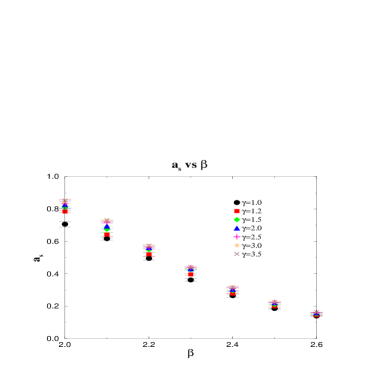
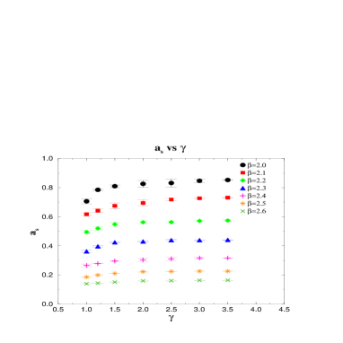
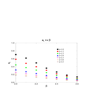
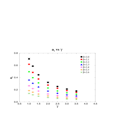
Figure 5: $a_{s}$ vs $\beta$, $a_{s}$ vs $\gamma$, $a_{t}$ vs $\beta$ and $a_{t}$ vs $\gamma$

2.4 Monopole Action At Finite Temperature

Now let us construct the 4D effective monopole action at finite temperature adopting $N_{s}^{3}\times N_{t}$ ($N_{s}\gg N_{t}$) lattices. Here we have to consider spacelike monopole currents $k_{i}(i=1,2,3)$ and timelike monopole current $k_{4}$ separately. An abelian Wilson loop operator is expressed as

$$W_{a}=\exp\bigl{\{}i\sum_{s}J_{\mu}(s)\theta_{\mu}(s)\bigr{\}},$$ (27)

where $J_{\mu}(s)$ is an external current taking $\pm 1$ along the Wilson loop. Since $J_{\mu}(s)$ is conserved, it is rewritten for a simple flat Wilson loop in terms of an antisymmetric variable $M_{\mu\nu}(s)$ as $J_{\nu}(s)=\partial_{\mu}^{\prime}M_{\mu\nu}(s)$. $M_{\mu\nu}(s)$ takes $\pm 1$ on the surface with the Wilson loop boundary. Then we get

$$W_{a}=\exp\bigl{\{}-\frac{i}{2}\sum_{s}M_{\mu\nu}(s)\theta_{\mu\nu}(s)\bigr{\}},$$ (28)

where $\theta_{\mu\nu}(s)=\partial_{\mu}\theta_{\nu}(s)-\partial_{\nu}\theta_{\mu}(s)$. Using the decomposition $\theta_{\mu\nu}(s)=\bar{\theta}_{\mu\nu}(s)+2\pi n_{\mu\nu}(s)$, we get

$$W_{a} = W_{p}\cdot W_{m},$$ (29)

$$W_{p} = \exp\bigl{\{}-i\sum_{s,s^{\prime}}\partial_{\mu}^{\prime}\bar{\theta}_{\mu\nu}(s)D(s-s^{\prime})J_{\nu}(s^{\prime})\bigr{\}},$$ (30)

$$W_{m} = \exp\bigl{\{}2\pi i\sum_{s,s^{\prime}}k_{\beta}(s)D(s-s^{\prime})\frac{1}{2}\epsilon_{\alpha\beta\rho\sigma}\partial_{\alpha}M_{\rho\sigma}(s^{\prime})\bigr{\}},$$ (31)

where $D(s)$ is the lattice Coulomb propagator [30]. Since $\partial_{\mu}^{\prime}\bar{\theta}_{\mu\nu}(s)$ contains only the photon fields, $W_{p}$ ($W_{m}$) is the photon (monopole) contribution to the Wilson loop. An ordinary space-time Wilson loop has a contribution only from spacelike monopoles, whereas both space and timelike monopoles contribute to a spacelike Wilson loop. The physical string tension has a finite value in the confinement phase but it is zero in the deconfinement phase. On the other hand, the spatial string tension determined by the spacelike Wilson loop has a finite value in both phases. Another special feature of the monopole action at finite temperature comes from the finite size in the time direction. We define a blockspin transformation of monopole currents [31] as

$$K_{\mu\neq 4}(s_{s},s_{4}) = \sum_{i,j=0}^{n_{s}-1}\sum_{l=0}^{n_{t}-1}k_{\mu\neq 4}\bigl{(}n_{s}s_{s}+(n_{s}-1)\hat{\mu}+i\hat{\nu}+j\hat{\rho},n_{t}s_{4}+l\bigr{)},$$ (32)

$$K_{4}(s_{s},s_{4}) = \sum_{i,j,l=0}^{n_{s}-1}k_{4}\bigl{(}n_{s}s_{s}+i\hat{\mu}+j\hat{\nu}+l\hat{\rho},n_{t}s_{4}+(n_{t}-1)\bigr{)},$$ (33)

where $n_{s}$ ($n_{t}$) is a blockspin factor for space (time) direction. Actually, we consider mostly the $n_{t}=1$ case.

2.5 Results

The parameters used in the simulations and the corresponding lattice spacing ($a_{s},a_{t}$) are summarized in Table 3. The lattice sizes and the temperatures are written in Table 3. We perform 6000 thermalization sweeps and take 40 configurations totally at every 100 sweeps. The inverse Monte-Carlo method used here is the modified Swendsen’s method extended to monopole currents with the conservation law (see Appendix A.2) [9, 30]. For simplicity, we assume that the effective monopole action is composed of only quadratic interactions. We adopts 84 interactions (For the explicit definition of each interaction, see Appendix B.1).

$\beta$	$\gamma$	$a_{s}$	$a_{t}$
2.470	2.841	0.250	0.075
2.500	2.615	0.225	0.075
2.533	2.354	0.200	0.075
2.548	2.256	0.190	0.075
2.565	2.152	0.180	0.075
2.573	2.098	0.175	0.075
2.581	2.042	0.170	0.075
2.598	1.927	0.160	0.075

Table 2: Parameter ($\beta$ , $\gamma$) and lattice spacing ($a_{s}$, $a_{t}$).

T	Lattice size	$N_{t}a_{t}(=\frac{1}{T})$
$0.6T_{c}$	$72^{3}\times 32$	$2.4$
$0.8T_{c}$	$72^{3}\times 24$	$1.8$
$0.96T_{c}$	$72^{3}\times 20$	$1.5$
$1.2T_{c}$	$72^{3}\times 16$	$1.2$
$1.6T_{c}$	$72^{3}\times 12$	$0.9$
$2.4T_{c}$	$72^{3}\times 8$	$0.6$

Table 3: Temperature, lattice size and $N_{t}a_{t}$.

Figure 6: The couplings vs $N_{s}$ for $b_{s}=1.5$. $T=0.8T_{c}$(left) and $T=1.2T_{c}$(right).

First to get the infinite-volume limit, we determine the actions for different lattice sizes at each ($\beta$, $\gamma$) and temperatures. We consider two different lattice sizes. The data show that the volume dependence is hardly seen. The examples for $b_{s}=1.5$ and $T=0.8T_{c}$, $1.2T_{c}$ are shown in Fig. 6.

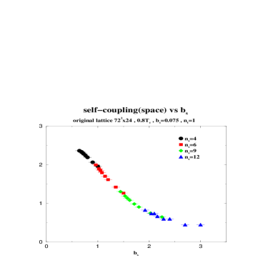
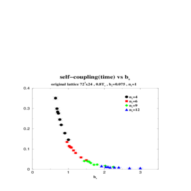
Figure 7: $n_{s}$-dependence of the couplings $f_{1}$(left) and $f_{2}$(right) at $0.8T_{c}$.

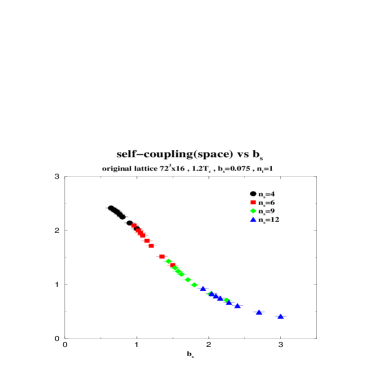
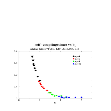
Figure 8: $n_{s}$-dependence of the couplings $f_{1}$(left) and $f_{2}$(right) at $1.2T_{c}$.

To get the continuum limit for space directions, we perform the blockspin transformation ($n_{s}=4,6,9,12$) for each temperature. The $n_{s}$-dependences of the couplings $f_{1}$ and $f_{2}$ for $0.8T_{c}$ and $1.2T_{c}$ are shown in Fig. 7 and Fig. 8. These figures indicate $n_{s}$-independence. The data of the couplings f1 and f2 for all temperatures are seen in Fig. 9. We can see the nice scaling behaviors at each temperature.

Figure 9: Temperature and $b_{s}$ dependence of self-couplings for spacelike monopole (left) and timelike monopole (right).

$N_{t}$	$\beta$	$\gamma$	$a_{s}$	$a_{t}$
20	2.446	2.400	0.250	0.090
	2.497	2.200	0.225	0.090
	2.532	1.981	0.200	0.090
	2.564	1.750	0.175	0.090
$N_{t}$	$\beta$	$\gamma$	$a_{s}$	$a_{t}$
16	2.462	1.942	0.250	0.113
	2.490	1.767	0.225	0.113
	2.519	1.607	0.200	0.113
	2.552	1.450	0.175	0.113

Table 4: Parameters to see the $N_{t}$-dependence at $0.8T_{c}$.

$N_{t}$	$\beta$	$\gamma$	$a_{s}$	$a_{t}$
12	2.465	2.178	0.250	0.100
	2.496	1.985	0.225	0.100
	2.525	1.781	0.200	0.100
	2.558	1.598	0.175	0.100
$N_{t}$	$\beta$	$\gamma$	$a_{s}$	$a_{t}$
8	2.450	1.509	0.250	0.151
	2.476	1.386	0.225	0.151
	2.504	1.262	0.200	0.151
	2.534	1.131	0.175	0.151

Table 5: Parameters to see the $N_{t}$-dependence at $1.2T_{c}$.

Figure 10: $N_{t}$-dependence for some couplings at $b_{s}=1.2$, $T=0.8Tc$.

Figure 11: $N_{t}$-dependence for some couplings at $b_{s}=1.2$, $T=1.2T_{c}$.

Figure 12: $N_{t}$ and $b_{s}$ dependence of self-couplings for spacelike monopole (left) and timelike monopole (right) at $0.8Tc$.

Figure 13: $N_{t}$ and $b_{s}$ dependence of self-couplings for spacelike monopole (left) and timelike monopole (right) at $1.2Tc$.

Next let us discuss the continuum limit in the time direction, studying $N_{t}$-dependence of the actions. The parameters used in different $N_{t}$ are in Table 5 ($0.8T_{c}$) and in Table 5 ($1.2T_{c}$). Figures 11 and 11 show $N_{t}$-independence of the actions for $N_{t}\geq 20$ (at $T=0.8T_{c}$) and $N_{t}\geq 12$ (at $T=1.2T_{c}$). The data for all $b_{s}$ are plotted in Fig. 12 ($0.8T_{c}$) and in Fig. 13 ($1.2T_{c}$). Because the temperatures are fixed, this means $a_{t}$-independence also.

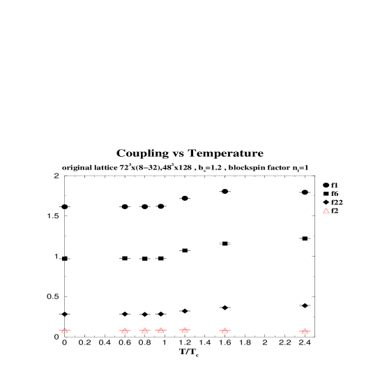
Figure 14: Temperature dependence for f1, f6, f22 (space) and f2 (time) at $b_{s}=1.2$

Figure 15: Distance-dependence of the couplings apart in the space direction. Left is the spacelike monopole case and right is the timelike monopole case at $0.8Tc$, $b_{s}=0.8$.

Figure 16: Distance-dependence of the couplings apart in the time direction. Left is the spacelike monopole case and right is the timelike monopole case at $0.8Tc$, $b_{s}=0.8$.

The features of the almost perfect monopole action at finite temperature are the following: (1) Perpendicular interactions are found to be negligible. We can discuss spacelike and timelike monopole actions separately. (2) Fig. 9 and Fig. 14 show that interactions of spacelike monopoles have no temperature-dependence in the confinement phase but have an obvious dependence in the deconfinement phase. On the other hand, interactions of timelike monopoles have no temperature-dependence in both phases. (3) We can examine the critical temperature $T_{c}$ of the confinement-deconfinement phase transition from the change of spacelike monopole interactions (Fig. 14). (4) The distance-dependence of the couplings is shown in Fig. 15 and Fig. 16. In both type of monopole actions, the self-coupling $f1$ (in the spacelike case) and $f2$ (in the timelike case) are dominant. The interactions between distant currents and perpendicular currents are very small except $f_{20}$. The coupling $f_{20}$ may get any truncation error. The couplings apart in the time direction (Fig. 16) are larger than the ones apart in the space direction (Fig. 15), because the lattice is anisotropic and the lattice distance in the space direction ($b_{s}$) is larger than the one in the time direction ($a_{t}$). Moreover, the extended timelike monopole is defined on the $b_{s}^{3}$ cube, whereas the extended spacelike monopole is defined on the $b_{s}^{2}a_{t}$ volume. If we consider both monopoles using the same scale, both couplings are of the same order [14].

In the confinement phase, the monopole currents form a long connected loop, but there appear only small loops in the deconfinement phase [14]. It seems that the temperature-dependence of the spacelike monopoles corresponds to the change of monopole current configurations. However, we can not yet find a key explanation of the confinement-deconfinement mechanism due to the spacelike monopoles, since the change of the spacelike monopole actions is not so drastic.

3 Monopole Action At High Temperature

3.1 The Dimensional Reduction

In this section we consider the effective monopole action beyond the critical temperature and investigate the origin of the nonperturbative effect in the deconfinement phase.

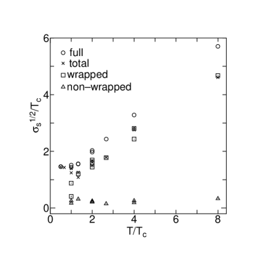
Figure 17: The full (non-abelian) spatial string tension (circle), the total monopole contribution (cross), the wrapped monopole contribution (square) and the non-wrapped monopole contribution (triangle). This figure is taken from Ref. [17].

The relations between the monopoles and the spatial string tension in (SU(2))_4D have been studied and the interesting features are observed [13, 17]. The data of the spatial string tensions in Ref. [17] is shown in Fig. 17. These data suggest that we can understand the nonperturbative effects in the deconfinement phase by the dynamics of the timelike monopoles.

To study the roles of the timelike monopoles, we consider the dimensional reduction. 4D timelike monopoles become instantons in $(GG)_{3D}$. It has a classical solution with a magnetic charge — ’t Hooft-Polyakov monopole (instanton) [18, 19].
Polyakov showed analytically that under the dilute Coulomb gas approximation of the ’t Hooft-Polyakov instantons, the string tension has a finite value [20]. The validity of the approximation has been proved by numerical simulations in the London limit [21]. The instantons in $(GG)_{3D}$ play a very important role for the nonperturbative effects like the string tension. It is expected that the mechanism reproducing the spatial string tension in (SU(2))_4D at high temperature is the same as that in $(GG)_{3D}$.

The starting point of the dimensional reduction is the action of (SU(2))_4D at finite temperature.

$$S = \int_{0}^{\beta}dx\int d^{3}x\frac{1}{4}F_{\mu\nu}^{a}F_{\mu\nu}^{a},$$ (34)

$$F_{\mu\nu}^{a} = \partial_{\mu}A_{\nu}^{a}-\partial_{\nu}A_{\mu}^{a}-gf_{abc}A_{\mu}^{b}A_{\nu}^{c}.$$ (35)

At high temperature region after performing the dimensional reduction, the action (34) is described by $(GG)_{3D}$ with the following action [5] :

$$S_{eff}=\int d^{3}x\Bigl{\{}\frac{1}{4}F_{ij}^{a}F_{ij}^{a}+\frac{1}{2}\bigl{(}D_{i}A_{0}^{a}\bigr{)}^{2}+\frac{1}{2}m_{D0}^{2}A_{0}^{a}A_{0}^{a}+\lambda_{A}\bigl{(}A_{0}^{a}A_{0}^{a}\bigr{)}^{2}\Bigr{\}}.$$ (36)

The 2-loop calculations give us the relations between the parameters appearing in (36) and those of the original action (34) [5] :

$$g_{3}^{2} = g^{2}(\mu)T\bigl{[}1+\frac{g^{2}}{16\pi^{2}}(\frac{44}{3}\frac{\mu}{\mu_{T}}+\frac{2}{3})\bigr{]},$$ (37)

$$m_{D0}^{2} = \frac{2}{3}g^{2}(\mu)T^{2}\bigl{[}1+\frac{g^{2}}{16\pi^{2}}(\frac{44}{3}\frac{\mu}{\mu_{T}}+\frac{10}{3})\bigr{]},$$ (38)

$$\lambda_{A} = \frac{g^{4}(\mu)T}{3\pi^{2}}\bigl{[}1+2\frac{g^{2}}{16\pi^{2}}(\frac{44}{3}\frac{\mu}{\mu_{T}}+\frac{7}{3})\bigr{]},$$ (39)

where $g^{2}(\mu)$ is the 4D gauge coupling and $T$ is the temperature in (SU(2))_4D and $\mu_{T}\approx 7.0555T$. For convenience, we redefine the parameters [5] as

$$g_{3}^{2}\ \ ,\ \ x\equiv\frac{\lambda_{A}}{g_{3}^{2}}\ \ ,\ \ y\equiv\frac{m_{D0}^{2}}{g_{3}^{4}}.$$ (40)

After the redefinition the dimensionful parameter is the 3D gauge coupling $g_{3}^{2}$ only.

3.2 The 3-Dimensional SU(2) Georgi-Glashow Model On The Lattice

The lattice action for $(GG)_{3D}$ is expressed as

$$S_{(GG)_{3D}} = S_{G}+S_{A},$$ (41)

$$S_{G} = \beta_{3}\sum_{x,i>j}\Bigl{\{}1-\frac{1}{2}Tr\bigl{[}U_{i}(x)U_{j}(x+\hat{i})U_{i}^{\dagger}(x+\hat{j})U_{j}^{\dagger}(x)\bigr{]}\Bigr{\}},$$ (42)

$$S_{A} = \sum_{x,i}2\bigl{[}TraA_{0}^{2}(x)-TraA_{0}(x)U_{i}(x)A_{0}(x+\hat{i})U_{i}^{\dagger}(x)\bigr{]}$$ (43)

$$+ \sum_{x}\bigl{[}(\tilde{m}_{D0}a)^{2}TraA_{0}^{2}(x)+a\lambda_{A}\bigl{(}\frac{1}{2}TraA_{0}^{2}(x)\bigr{)}^{2}\bigr{]},$$

$$\beta_{3} = \frac{4}{g_{3}^{2}a},$$ (44)

where $a$ is the lattice spacing and $\tilde{m}_{D0}$ is the bare mass in the lattice scheme. In order to relate the results of lattice calculation in $(GG)_{3D}$ to the physics of the original (SU(2))_4D at high temperature, it is necessary to consider the relation between the bare mass $\tilde{m}_{D0}$ and the renormalized mass in the continuum theory. The bare mass $\tilde{m}_{D0}$ is rewritten in terms of $\beta$, $x$ and $y$ as shown in Refs. [5, 32] from the requirement that the renormalized mass in the lattice scheme is the same as the one in the $\overline{MS}$ scheme. The lattice action is finally expressed as follows:

$$S_{(GG)_{3D}} = S_{G}+S_{A},$$ (45)

$$S_{G} = \beta_{3}\sum_{x,i>j}\Bigl{\{}1-\frac{1}{2}Tr\bigl{[}U_{i}(x)U_{j}(x+\hat{i})U_{i}^{\dagger}(x+\hat{j})U_{j}^{\dagger}(x)\bigr{]}\Bigr{\}},$$ (46)

$$S_{A} = \beta_{3}\sum_{x,i}\frac{1}{2}Tr\bigl{[}\tilde{A_{0}}(x)U_{i}(x)\tilde{A_{0}}(x+\hat{i})U_{i}^{\dagger}(x)\bigr{]}$$ (47)

$$+ \sum_{x}\Bigl{\{}-\beta_{3}(3+\frac{1}{2}h)\frac{1}{2}Tr\tilde{A_{0}}^{2}(x)+\beta_{3}x\bigl{(}\frac{1}{2}Tr\tilde{A_{0}}^{2}(x)\bigr{)}^{2}\Bigr{\}},$$

$$\beta_{3} = \frac{4}{g_{3}^{2}a},$$ (48)

$$h \equiv \frac{16}{\beta_{3}^{2}}y-\frac{\Sigma(4+5x)}{\pi\beta_{3}}$$ (49)

$$- \frac{1}{\pi^{2}\beta_{3}^{2}}\Bigl{\{}(20x-10x^{2})(\ln\frac{3}{2}\beta_{3}+0.09)+8.7+11.6x\Bigr{\}},$$

where $\Sigma=3.1759114$ and $\tilde{A_{0}}$ is defined by $aA_{0}^{2}=\beta_{3}\tilde{A_{0}}^{2}/4$ .

To compare the effective monopole action of (SU(2))_4D with that of $(GG)_{3D}$, we should take the same scale in both theories. A lattice spacing in $(GG)_{3D}$ is controlled by a parameter $\beta_{3}$ and is given in unit of $g_{3}^{2}$ as

$$a=\frac{4}{g_{3}^{2}\beta_{3}}.$$ (50)

The relation between the 3D gauge coupling $g_{3}$ and the 4D gauge coupling $g(T)$ which depends on temperature $T$ in the 1-loop calculation is

$$g_{3}^{2}=g^{2}(T)T.$$ (51)

The 4D gauge coupling $g(T)$ have been determined from the temperature-dependence of the spatial string tension in (SU(2))_4D in the 1-loop calculation [33]:

$$\sqrt{\sigma_{s}(T)} = (0.334\pm 0.014)g^{2}(T)T,$$ (52)

$$g^{-2}(T) = \frac{11}{12\pi^{2}}\ln\frac{T}{\Lambda_{T}},$$ (53)

$$\Lambda_{T} = 0.050(10)T_{c}.$$ (54)

The string tension of the dimensional reduced $(GG)_{3D}$ have been measured in Ref. [6] and the value is fitted well only in terms of the gauge coupling as $\sqrt{\sigma_{(GG)_{3D}}}=0.326(7)g_{3}^{2}$. This means that $\sqrt{\sigma_{s}(T)}$ is almost the same as $\sqrt{\sigma_{(GG)_{3D}}}$ numerically. Using the 4D gauge coupling, the lattice spacing is rewritten in unit of the temperature $T$ as

$$a=\frac{4}{g_{3}^{2}\beta_{3}}=\frac{4}{g^{2}(T)T\beta_{3}}.$$ (55)

We also use the relation between the critical temperature $T_{c}$ and the (zero temperature) 4D physical string tension $\sigma_{phys}$  [34] :

$$\frac{T_{c}}{\sqrt{\sigma_{phys}}}=0.69\pm 0.02.$$ (56)

Hence we can determine the lattice spacing $a$ in $(GG)_{3D}$ for each $T$ in unit of the square root of the (zero temperature) 4D physical string tension.

3.3 Results

Based on the method in Ref. [35], we perform Monte-Carlo simulations of $(GG)_{3D}$. Before the comparison of both actions, we measure the string tension. To evaluate the contribution of the instantons to the string tension, we define the instantons in $(GG)_{3D}$. The methods for the abelian projection and the decomposition of the U(1) plaquette variables are the same as in (SU(2))_4D [21]. After the decomposition we can define an instanton as

$$k(s)=-\frac{1}{2}\epsilon_{ijk}\partial_{i}n_{jk}(s),(i,j,k=1,2,3),$$ (57)

and the instanton part of the Wilson loop in 3D is expressed as

$$W_{3d-m}=\exp\Bigl{\{}2\pi i\sum_{s,s^{\prime}}k(s)D(s-s^{\prime})\frac{1}{2}\epsilon_{ijk}\partial_{i}M_{jk}(s^{\prime})\Bigr{\}}.$$ (58)

$a$	$\beta_{3}$	$x$	$h$
0.160	6.394	0.010	-0.658
0.170	6.018	0.010	-0.696
0.175	5.846	0.010	-0.714
0.180	5.683	0.010	-0.732
0.190	5.384	0.010	-0.769
0.200	5.115	0.010	-0.805
0.225	4.547	0.010	-0.892
0.250	4.092	0.010	-0.977

Table 6: The parameters in $(GG)_{3D}$ corresponding to the lattice spacing $a$ at $1.92T_{c}$ in (SU(2))_4D.

$a$	$\beta_{3}$	$x$	$h$
0.160	5.428	0.094	-0.749
0.170	5.109	0.094	-0.790
0.175	4.963	0.094	-0.810
0.180	4.825	0.094	-0.830
0.190	4.571	0.094	-0.870
0.200	4.342	0.094	-0.909
0.225	3.860	0.094	-1.002
0.250	3.474	0.094	-1.091

Table 7: The parameters in $(GG)_{3D}$ corresponding to the lattice spacing $a$ at $2.4T_{c}$ in (SU(2))_4D.

$a$	$\beta_{3}$	$x$	$h$
0.160	3.200	0.079	-1.068
0.170	3.012	0.079	-1.113
0.175	2.926	0.079	-1.134
0.180	2.844	0.079	-1.154
0.190	2.695	0.079	-1.193
0.200	2.560	0.079	-1.230
0.225	2.276	0.079	-1.308
0.250	2.048	0.079	-1.370

Table 8: The parameters in $(GG)_{3D}$ corresponding to the lattice spacing $a$ at $4.8T_{c}$ in (SU(2))_4D.

T	Lattice size	Lattice size
	(4DSU(2))	($(GG)_{3D}$)
$1.92T_{c}$	$48^{3}\times 10$	$48^{3}$
$2.4T_{c}$	$48^{3}\times 8$	$48^{3}$
$4.8T_{c}$	$48^{3}\times 4$	$48^{3}$

Table 9: Temperature and Lattice size for (SU(2))_4D and $(GG)_{3D}$

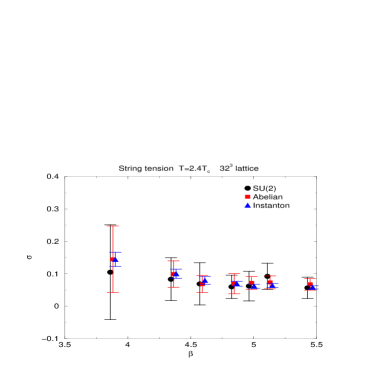
Figure 18: The string tension of $(GG)_{3D}$ at $2.4T_{c}$.

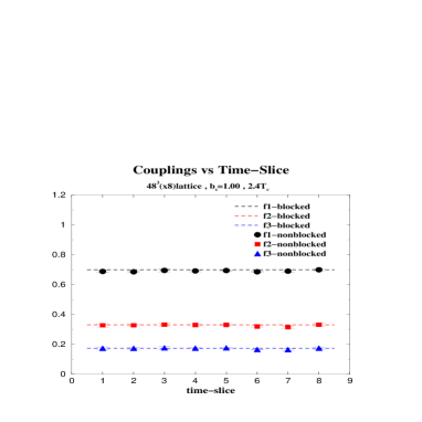
Figure 19: Comparing the timelike monopole action at $2.4T_{c}$.

The parameters used in the measurements of the string tension are determined by the above-mentioned procedure and are summarized in Tables 7–9. The lattice sizes are summarized in Table 9. To get the string tensions we fit the static potential (24) with the function $\sigma R+\alpha\log R+c$ (where $\alpha$ and $c$ are constants). The results in Fig. 19 show that the abelian dominance and the instanton dominance for the string tension hold good.

Since the instanton dominance is observed, we try to derive effective instanton actions in $(GG)_{3D}$ and compare those actions with the timelike monopole actions in (SU(2))_4D in the deconfinement phase. For the comparison, we have to choose the time-slice in the 4D case.

Figure 20: The relation between the couplings and distance at $2.4T_{c}$.

However at high temperature the timelike monopoles are almost in wrapped monopole loops and the obtained actions at each time-slice are expected to be same. This is seen actually as shown in Fig.19. So in (SU(2))_4D we may use the timelike monopoles after blockspin transformations completely in the time direction. Here to perform the blockspin transformation means an averaging of the timelike monopoles at each time-slice.

Because there is no conservation law in the instanton case, we use the original Swendsen’s method [36] to determine instanton actions (see Appendix A.1). We assume that the instanton actions have 2-point interactions only and adopt 10 interactions within the distance 3 in unit of lattice spacing.

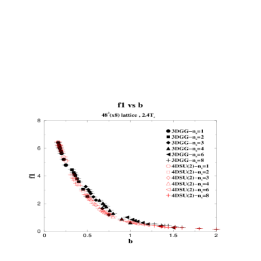
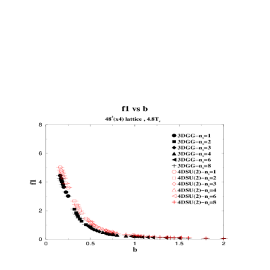
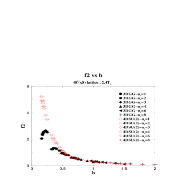
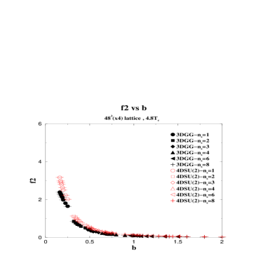
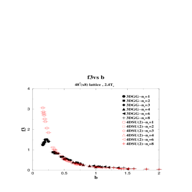
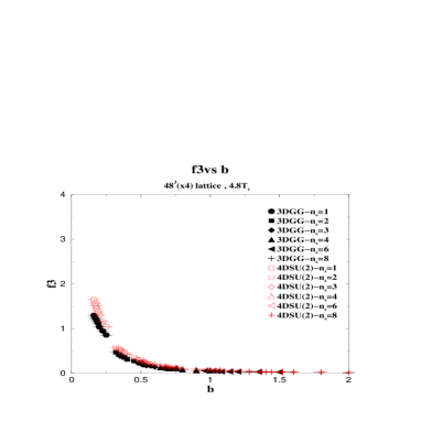
Figure 21: Coupling $f_{1}$(top), $f_{2}$(middle) and $f_{3}$(bottom) at $2.4T_{c}$(left column) and $4.8T_{c}$(right column).

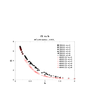
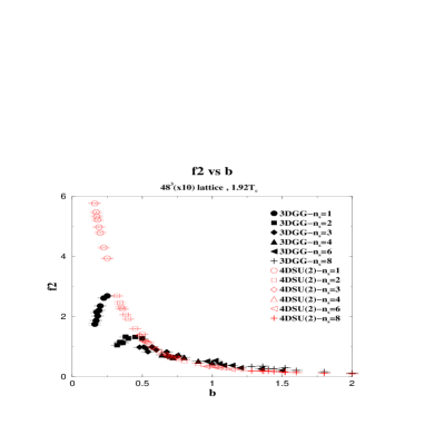
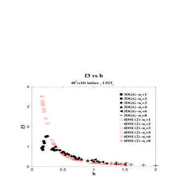
Figure 22: Coupling $f_{1}$(left), $f_{2}$(right) and $f_{3}$(bottom) at $1.92T_{c}$.

In Fig. 20 we show the distance-dependence of the couplings at $b=$0.25, 0.50, 0.75, 1.00, 1.50 and 2.00 for $T=2.4T_{c}$. The couplings of the 3D instanton action are different from those of the 4D timelike monopole action at small $b$ regions, especially in the case of the blockspin factor $n_{s}=1$. However when we perform the blockspin transformation, both couplings tend to be the same. To see the scaling behavior, we show the $n_{s}$-dependence of the couplings for both actions for different temperature in Fig. 21, 22. These figures show the good scaling behaviors for the couplings $f_{1}$, $f_{2}$ and $f_{3}$ in both actions, especially for $b>0.4(\sqrt{\sigma})^{-1}$. From these figures it turns out that the couplings of the monopole actions originated from (SU(2))_4D and those of the instanton actions in $(GG)_{3D}$ flow on the same renormalized trajectories in the large $b$ region at $T\geq 2.4T_{c}$. In Fig. 21 we also show the case of $4.8T_{c}$. The scaling behaviors look good and the agreement of both couplings is much better than that for $2.4T_{c}$. On the other hand, the couplings at $1.92T_{c}$ are shown in Fig. 22. The figure shows that the couplings of both actions have a nice scaling at large $b$ region, but both actions do not coincide. The temperature $T=1.92T_{c}$ is so small that we can not apply the dimensional reduction. The dimensional reduction works well at $T\geq 2.4T_{c}$ region also in the framework of the monopole (instanton) action representing nonperturbative effects.

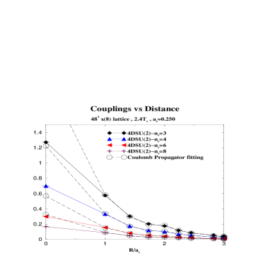
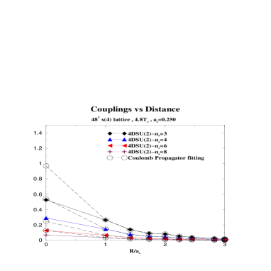
Figure 23: The fitting of the 3-dimensional timelike monopole actions by the Coulomb propagator at $2.4T_{c}$ (left) and $4.8T_{c}$ (right).

Since we have obtained the monopole (instanton) action both in (SU(2))_4D and in $(GG)_{3D}$, we consider the property of the actions. As Polyakov showed in Ref. [20], if instantons behave as a Coulomb gas, the string tension has a non-zero finite value. In order to explain the nonperturbative effect in the deconfinement phase such as the spatial string tension by instantons, we compare the obtained monopole (instanton) action with that of the Coulomb gas. Using the method in Ref. [21], we fit the timelike monopole action obtained from (SU(2))_4D by the 3D lattice Coulomb propagator. When we define the lattice Coulomb propagator as

$$\Delta_{L}^{-1}(s-s^{\prime})=C_{1}\delta^{3}(s-s^{\prime})+C_{2}\sum_{i}\delta^{3}(s-(s^{\prime}+\hat{i}))+...,$$ (59)

we get a beautiful fit

$$f_{i}\sim Const.\times C_{i}(i\neq 1)$$ (60)

at $T=2.4T_{c}$ and $T=4.8T_{c}$ as shown in Fig. 23. Here {$f_{i}$} are the couplings of the timelike monopole (instanton) action and the detail is shown in Appendix B.2. The results obtained here are very similar in Ref. [21]. So we can conclude that the timelike monopoles (instantons) behave as a Coulomb gas. This fact means that monopoles in the deconfinement phase form a Coulomb gas of the wrapped monopole loops and reproduce the spatial string tension.

4 Concluding Remarks

We have studied the effective monopole action at finite temperature in (SU(2))_4D. (1) We have determined the anisotropy $\xi$ and the lattice spacings $a_{s}$ and $a_{t}$ for various $(\beta,\gamma)$ on the anisotropic lattices in (SU(2))_4D. Using the relations between the parameters $(\beta,\gamma)$ and the lattice spacing $(a_{s},a_{t})$, the thermalized monopole current configurations are generated for various temperatures $(T\leq 4.8T_{c})$ in MA gauge. After performing the blockspin transformations for space directions, we have obtained the almost perfect 4-dimensional effective monopole action under the assumption of two-point interactions alone. The action depends only on the physical scale $b_{s}$ and the temperature $T$. The temperature-dependence of the action appear with respect to the spacelike monopole couplings in the deconfinement phase, whereas the timelike monopole couplings have no temperature-dependence. (2) In $(GG)_{3D}$, we have calculated the string tensions from the non-abelian, abelian and instanton Wilson loops at the parameter regions obtained from the dimensional reduction of (SU(2))_4D. The abelian dominance and the monopole dominance have been observed also. Instantons play an important role for the infrared physics in $(GG)_{3D}$. (3) At high temperature (the deconfinement phase) in (SU(2))_4D, we have determined the 3-dimensional effective monopole action from $(GG)_{3D}$. We compare the action with the timelike monopole action which is obtained from (SU(2))_4D at the same temperature. The results show that both actions agree very well at large $b$ region for $T\geq 2.4T_{c}$. The dimensional reduction works well for the infrared physics also in the monopole-instanton picture. The timelike monopole (instanton) actions here obtained are fitted beautifully by the lattice Coulomb propagator. The result means that in the deconfinement phase, the mechanism reproducing the spatial string tension is the same as the one of $(GG)_{3D}$. Namely the Coulomb gas of the wrapped monopole loops induce the nonperturbative effects such as the spatial string tension. Although the dimensional reduction works good only for $T\geq 2.4T_{c}$, the 4D timelike monopole actions for $T<2.4T_{c}$ are very similar to the ones for $T\geq 2.4T_{c}$. The nonperturbative effects in the deconfinement phase are given by the timelike monopoles in (SU(2))_4D.

The following subjects are very interesting to be studied. (1) The exact mechanism of the confinement-deconfinement transition should be clarified. From the numerical study of critical exponents, spacelike monopoles play a key role in the mechanism. But we have not yet known what mechanism of spacelike monopoles is responsible for the transition. Simple energy-entropy arguments may not be true, since the energy of the system (which is well approximated by the self coupling of the monopole action) decreases monotonously as $b_{s}$ becomes larger even in the deconfinement phase. If the entropy is governed by a kinematical factor which does not depend on $b_{s}$ as in the zero-temperature case, energy-entropy arguments can not explain the transition. (2) It is interesting to transform the obtained actions into those of different models like a dual abelian Higgs model or a string model. We may get a different viewpoint with respect to the mechanism of the deconfinement transition. (3) To study all nonperturbative effects such as Debye-screening mass and glueball mass is also interesting. Are they all explained by monopoles?

Appendix A Inverse Monte-Carlo Methods

A.1 The Original Swendsen’s Method

We apply the original Swendsen’s method [36] to determine the 3D instanton action from the thermalized instanton configurations. The partition function of the theory described by the instantons is given by the following.

$$Z=\Bigl{(}\prod_{s}\sum_{k(s)=-\infty}^{\infty}\Bigr{)}\exp\bigl{(}-S[k]\bigr{)},$$ (61)

where $S[k]$ is an instanton action. The action may be written as a linear combination of all independent operators which are summed over the whole lattice. We denote each operator as $S_{i}[k]$. Then the action may be expressed as follows:

$$S[k]=\sum_{i}f_{i}S_{i}[k],$$ (62)

where $f_{i}$ are coupling constants. The expectation value of some operator $O[k]$ is written by

$$\Bigl{\langle}O[k]\Bigr{\rangle}=\frac{1}{Z}\Bigl{(}\prod_{s}\sum_{k(s)=-\infty}^{\infty}\Bigr{)}O[k]\exp\bigl{(}-S[k]\bigr{)}.$$ (63)

Let us focus on a site $s^{\prime}$ and define $\hat{S}[k]$ which contains $k(s\prime)$. We get

$$\Bigl{\langle}O[k]\Bigr{\rangle}=\frac{1}{Z}\Bigl{(}{\prod_{s}}^{\prime}\sum_{k(s)=-\infty}^{\infty}\Bigr{)}\exp\bigl{\{}-(S[k]-\hat{S}[k])\bigr{\}}\sum_{k(s^{\prime})=-\infty}^{\infty}O[\hat{k},\{k\}^{\prime}]\exp\bigl{(}-\hat{S}[k]\bigr{)},$$ (64)

where $\prod^{\prime}$ means the product except the site $s^{\prime}$ and $\hat{k}=k(s^{\prime})$ and $\{k\}^{\prime}$ is the coset of $\hat{k}$. We rewrite Eq.(64) as

$$\Bigl{\langle}O[k]\Bigr{\rangle} = \frac{1}{Z}\Bigl{(}\prod_{s}\sum_{k(s)=-\infty}^{\infty}\Bigr{)}\frac{\sum_{\hat{k}=-\infty}^{\infty}O[\hat{k},\{k\}^{\prime}]\exp\bigl{\{}-\hat{S}[\hat{k},\{k\}^{\prime}]\bigr{\}}}{\sum_{\hat{k}=-\infty}^{\infty}\exp\bigl{\{}-\hat{S}[\hat{k},\{k\}^{\prime}]\bigr{\}}}\exp\bigl{(}-S[k]\bigr{)}$$ (65)

$$\equiv \Bigl{\langle}\hat{O}[k]\Bigr{\rangle},$$ (66)

where

$$\hat{O}[k]\equiv\frac{\sum_{\hat{k}=-\infty}^{\infty}O[\hat{k},\{k\}^{\prime}]\exp\bigl{\{}-\hat{S}[\hat{k},\{k\}^{\prime}]\bigr{\}}}{\sum_{\hat{k}=-\infty}^{\infty}\exp\bigl{\{}-\hat{S}[\hat{k},\{k\}^{\prime}]\bigr{\}}}.$$ (67)

When we use the definition of the instanton by DeGrand-Toussaint [24], the sum with respect to $\hat{k}$ change from $[-\infty,\infty]$ to $[-(3n^{2}-1),3n^{2}-1]$ where n is a factor of blockspin transformation of instantons. Using the identity Eq.(66), let us determine the instanton action iteratively. Since we don’t know the correct set of coupling constants $\{f_{i}\}$, we start from trial coupling constants $\{\tilde{f}_{i}\}$. We define $\bar{O}$ in which the true coupling constants $\{f_{i}\}$ in Eq.(67) are replaced by the trial ones $\{\tilde{f}_{i}\}$ as

$$\bar{O}[k]=\frac{\sum_{\hat{k}=k_{min}}^{k_{max}}O[\hat{k},\{k\}^{\prime}]\exp\bigl{\{}-\sum_{i}\tilde{f}_{i}\hat{S}_{i}[\hat{k},\{k\}^{\prime}]\bigr{\}}}{\sum_{\hat{k}=k_{min}}^{k_{max}}\exp\bigl{\{}-\sum_{i}\tilde{f}_{i}\hat{S}_{i}[\hat{k},\{k\}^{\prime}]\bigr{\}}}.$$ (68)

When $f_{i}$ is not equal to $\tilde{f}_{i}$ for all $i$, $\Bigl{\langle}O[k]\Bigr{\rangle}\neq\Bigl{\langle}\bar{O}[k]\Bigr{\rangle}$. But when $\{\tilde{f}_{i}\}$ are not far from $\{f_{i}\}$, we get the following expansion:

$$\Bigl{\langle}O[k]-\bar{O}[k]\Bigr{\rangle}\sim\sum_{i}\Bigl{\langle}\bar{O}\bar{S}_{i}-\overline{OS}_{i}\Bigr{\rangle}\bigl{(}f_{i}-\tilde{f}_{i}\bigr{)}.$$ (69)

In practice, we use $S_{i}[k]$ as an operator $O[k]$ to get a good convergence. Hence we get linear equations for $\{f_{i}\}$ as

$$\Bigl{\langle}S_{i}[k]-\bar{S}_{i}[k]\Bigr{\rangle}\sim\sum_{j}\Bigl{\langle}\bar{S}_{i}\bar{S}_{j}-\overline{S_{i}S_{j}}\Bigr{\rangle}\bigl{(}f_{j}-\tilde{f}_{j}\bigr{)}.$$ (70)

Starting from trial couplings $\{\tilde{f}_{i}\}$, we first calculate the expectation value $\Bigl{\langle}S_{i}[k]-\bar{S}_{i}[k]\Bigr{\rangle}$ using the instanton configurations. If the values of $\Bigl{\langle}S_{i}[k]-\bar{S}_{i}[k]\Bigr{\rangle}$ for all i are regarded as zero, $\{\tilde{f}_{i}\}$ can be adopted as the true coupling constants. If not, we solve Eq.(70) with respect to $\{f_{i}\}$ and adopt the solution $\{f_{i}\}$ as new trial couplings. Repeating the above-mentioned procedure we can obtain the true coupling constants and determine the instanton action iteratively.

A.2 The Modified Swendsen’s Method

The modified Swendsen’s Method [9, 10] is applied to determine the action of monopoles with current conservation law. So we use the method to determine the 4-dimensional effective monopole action.

The partition function of the theory is written as

$$Z=\Bigl{(}\prod_{s,\mu}\sum_{k_{\mu}(s)=-\infty}^{\infty}\Bigr{)}\Bigl{(}\prod_{s}\delta_{\partial_{\mu}^{\prime}k_{\mu}(s),0}\Bigr{)}\exp\bigl{(}-S[k]\bigr{)}.$$ (71)

Using the expression of Eq.(71), we consider the expectation value of some operator $O[k]$ which is written by monopole currents

$$\Bigl{\langle}O[k]\Bigr{\rangle}=\frac{1}{Z}\Bigl{(}\prod_{s,\mu}\sum_{k_{\mu}(s)=-\infty}^{\infty}\Bigr{)}\Bigl{(}\prod_{s}\delta_{\partial_{\mu}^{\prime}k_{\mu}(s),0}\Bigr{)}O[k]\exp\bigl{(}-S[k]\bigr{)}.$$ (72)

Because of the existence of the current conservation laws, we focus on a plaquette $(s^{\prime},\hat{\mu}^{\prime},\hat{\nu}^{\prime})$ instead of a site $s^{\prime}$ and define $\hat{S}[k]$ as a part of $S[k]$ which contains currents along the plaquette, i.e. $\{k_{\mu^{\prime}}(s^{\prime}),k_{\nu^{\prime}}(s^{\prime}+\hat{\mu}^{\prime}),k_{\mu^{\prime}}(s^{\prime}+\hat{\nu}^{\prime}),k_{\nu^{\prime}}(s^{\prime})\}$. Then we get

$$\Bigl{\langle}O[k]\Bigr{\rangle} = \frac{1}{Z}\Bigl{(}{\prod_{s,\mu}}^{\prime}\sum_{k_{\mu}(s)=-\infty}^{\infty}\Bigr{)}\Bigl{(}{\prod_{s}}^{\prime}\delta_{\partial_{\mu}^{\prime}k_{\mu}(s),0}\Bigr{)}\exp\bigl{\{}-(S[k]-\hat{S}[k])\bigr{\}}$$ (73)

$$\times \sum_{k_{\mu^{\prime}}(s^{\prime})=-\infty}^{\infty}\sum_{k_{\nu^{\prime}}(s^{\prime}+\hat{\mu}^{\prime})=-\infty}^{\infty}\sum_{k_{\mu^{\prime}}(s^{\prime}+\hat{\nu}^{\prime})=-\infty}^{\infty}\sum_{k_{\nu^{\prime}}(s^{\prime})=-\infty}^{\infty}$$

$$\times \delta_{\partial_{\mu}^{\prime}k_{\mu}(s^{\prime}),0}\delta_{\partial_{\mu}^{\prime}k_{\mu}(s^{\prime}+\hat{\mu}^{\prime}),0}\delta_{\partial_{\mu}^{\prime}k_{\mu}(s^{\prime}+\hat{\nu}^{\prime}),0}\delta_{\partial_{\mu}^{\prime}k_{\mu}(s^{\prime}+\hat{\mu}^{\prime}+\hat{\nu}^{\prime}),0}$$

$$\times O[k]\exp\bigl{(}-\hat{S}[k]\bigr{)},$$

where ${\prod_{s,\mu}}^{\prime}$ and ${\prod_{s}}^{\prime}$ mean the product which excludes the links and the sites in the plaquette considered. One of the $\delta$-functions on the four sites in the plaquette can be replaced by $\delta_{\partial_{\mu}^{\prime}k_{\mu}(s^{\prime})+\partial_{\mu}^{\prime}k_{\mu}(s^{\prime}+\hat{\mu}^{\prime})+\partial_{\mu}^{\prime}k_{\mu}(s^{\prime}+\hat{\nu}^{\prime})+\partial_{\mu}^{\prime}k_{\mu}(s^{\prime}+\hat{\mu}^{\prime}+\hat{\nu}^{\prime}),0}$ and this $\delta$-function does not contain any current in the plaquette. Then Eq.(73) is expressed as

$$\Bigl{\langle}O[k]\Bigr{\rangle} = \frac{1}{Z}\Bigl{(}{\prod_{s,\mu}}^{\prime}\sum_{k_{\mu}(s)=-\infty}^{\infty}\Bigr{)}\Bigl{(}{\prod_{s}}^{\prime}\delta_{\partial_{\mu}^{\prime}k_{\mu}(s),0}\Bigr{)}\exp\bigl{\{}-(S[k]-\hat{S}[k])\bigr{\}}$$ (74)

$$\times \delta_{\partial_{\mu}^{\prime}k_{\mu}(s^{\prime})+\partial_{\mu}^{\prime}k_{\mu}(s^{\prime}+\hat{\mu}^{\prime})+\partial_{\mu}^{\prime}k_{\mu}(s^{\prime}+\hat{\nu}^{\prime})+\partial_{\mu}^{\prime}k_{\mu}(s^{\prime}+\hat{\mu}^{\prime}+\hat{\nu}^{\prime}),0}$$

$$\times \bigl{(}\sum\delta\bigr{)}_{k}O[\hat{k},\{k\}^{\prime}]\exp\bigl{(}-\hat{S}[k]\bigr{)},$$

where $\{k\}^{\prime}$ does not contain the four currents in the plaquette considered and

$$\bigl{(}\sum\delta\bigr{)}_{k} \equiv \sum_{k_{\mu^{\prime}}(s^{\prime})=-\infty}^{\infty}\sum_{k_{\nu^{\prime}}(s^{\prime}+\hat{\mu}^{\prime})=-\infty}^{\infty}\sum_{k_{\mu^{\prime}}(s^{\prime}+\hat{\nu}^{\prime})=-\infty}^{\infty}\sum_{k_{\nu^{\prime}}(s^{\prime})=-\infty}^{\infty}$$ (75)

$$\times \delta_{\partial_{\mu}^{\prime}k_{\mu}(s^{\prime}),0}\delta_{\partial_{\mu}^{\prime}k_{\mu}(s^{\prime}+\hat{\mu}^{\prime}),0}\delta_{\partial_{\mu}^{\prime}k_{\mu}(s^{\prime}+\hat{\nu}^{\prime}),0}.$$

Defining the operator $\hat{O}[\hat{k},\{k\}^{\prime}]$ as

$$\hat{O}[\hat{k},\{k\}^{\prime}]\equiv\frac{\bigl{(}\sum\delta\bigr{)}_{k}O[\hat{k},\{k\}^{\prime}]\exp\bigl{(}-\hat{S}[k]\bigr{)}}{\bigl{(}\sum\delta\bigr{)}_{k}\exp\bigl{(}-\hat{S}[k]\bigr{)}},$$ (76)

then we can rewrite Eq.(74) as

$$\Bigl{\langle}O[k]\Bigr{\rangle} = \frac{1}{Z}\Bigl{(}\prod_{s,\mu}\sum_{k_{\mu}(s)=-\infty}^{\infty}\Bigr{)}\Bigl{(}\prod_{s}\delta_{\partial_{\mu}^{\prime}k_{\mu}(s),0}\Bigr{)}\hat{O}[\hat{k},\{k\}^{\prime}]\exp\bigl{\{}-S[k]\bigr{\}}$$ (77)

$$= \Bigl{\langle}\hat{O}[k]\Bigr{\rangle}.$$ (78)

From the three $\delta$-functions in $\bigl{(}\sum\delta\bigr{)}_{k}$, there are three constraints for the four currents on the plaquette considered. Namely only one current of the four is independent. Define the independent variable $M$ and replace the current $\hat{k}_{\mu^{\prime}}(s^{\prime})$ as

$$\hat{k}_{\mu^{\prime}}(s^{\prime})=k_{\mu^{\prime}}(s^{\prime})+M.$$ (79)

Using the three constraints for the four currents, we get

$$\hat{k}_{\nu^{\prime}}(s^{\prime}) = k_{\nu^{\prime}}(s^{\prime})-M,$$ (80)

$$\hat{k}_{\mu^{\prime}}(s^{\prime}+\hat{\nu}^{\prime}) = k_{\mu^{\prime}}(s^{\prime}+\hat{\nu}^{\prime})-M,$$ (81)

$$\hat{k}_{\nu^{\prime}}(s^{\prime}+\hat{\mu}^{\prime}) = k_{\nu^{\prime}}(s^{\prime}+\hat{\mu}^{\prime})+M.$$ (82)

Here we use the relation

$$\sum_{M=-\infty}^{\infty}\delta_{\hat{k}_{\mu^{\prime}}(s^{\prime}),k_{\mu^{\prime}}(s^{\prime})+M}=1.$$ (83)

Then we can replace the sum with respect to $\hat{k}$ by the sum with respect to $M$. When we use the DeGrand-Toussaint monopole definition, the sum with respect to $M$ is restricted from $m_{1}$ to $m_{2}$ where

$$m_{1} = -(3n^{2}-1)-min\{k_{\mu^{\prime}}(s^{\prime}),k_{\nu^{\prime}}(s^{\prime}+\hat{\mu}^{\prime}),-k_{\mu^{\prime}}(s^{\prime}+\hat{\nu}^{\prime}),-k_{\nu^{\prime}}(s^{\prime})\},$$ (84)

$$m_{2} = (3n^{2}-1)-max\{k_{\mu^{\prime}}(s^{\prime}),k_{\nu^{\prime}}(s^{\prime}+\hat{\mu}^{\prime}),-k_{\mu^{\prime}}(s^{\prime}+\hat{\nu}^{\prime}),-k_{\nu^{\prime}}(s^{\prime})\},$$ (85)

and $n$ is a number of blockspin transformations for all directions. Hence we get another representation of Eq.(76) as

$$\hat{O}[k]=\frac{\sum_{M=m_{1}}^{m_{2}}O[\bar{k}]\exp\bigl{(}-\hat{S}[\bar{k}]\bigr{)}}{\sum_{M=m_{1}}^{m_{2}}\exp\bigl{(}-\hat{S}[\bar{k}]\bigr{)}},$$ (86)

where

$$\bar{k}_{\mu}(s)=k_{\mu}(s)+M(\delta_{s,s^{\prime}}\delta_{\mu,\mu^{\prime}}+\delta_{s,s^{\prime}+\hat{\mu}^{\prime}}\delta_{\mu,\nu^{\prime}}-\delta_{s,s^{\prime}+\hat{\nu}^{\prime}}\delta_{\mu,\mu^{\prime}}-\delta_{s,s^{\prime}}\delta_{\mu,\nu^{\prime}}).$$ (87)

So we get the identity as follows:

$$\Bigl{\langle}O[k]\Bigr{\rangle}=\Bigl{\langle}\hat{O}[k]\Bigr{\rangle}.$$ (88)

Using Eq.(88) and the same procedure in Appendix A.1, we can obtain the monopole action.

Appendix B The Quadratic Interactions Adopted

B.1 4D Effective Monopole Action

Some comments on the 4D effective monopole action are in order. (1) We have to distinguish spacelike monopoles from timelike monopoles. (2) The current conservation laws exist at all sites. Using the conservation laws, we replace short-distance perpendicular interactions in terms of parallel interactions as many as possible as done in the $T=0$ case [9]. (3) Monopole current configurations are generated on the anisotropic lattice.

We adopt 69 parallel- and 15 perpendicular-interactions in the following action :

$$S[k] = \sum_{i=1}^{84}f_{i}S_{i}.$$ (89)

The interactions are summarized in Table 10.

Table 10: The quadratic interactions used for the 4D effective monopole action.

$\left\{f_{i}\right\}$	distance	type	$\left\{f_{i}\right\}$	distance	type
$f_{1}$	(0,0,0,0)	$k_{i}(s)k_{i}(s)$	$f_{43}$	(0,2,1,1)	$k_{i}(s)k_{i}(s+2\hat{j}+\hat{l}+\hat{4})$
$f_{2}$	(0,0,0,0)	$k_{4}(s)k_{4}(s)$	$f_{44}$	(0,2,1,1)	$k_{i}(s)k_{i}(s+\hat{j}+\hat{l}+2\hat{4})$
$f_{3}$	(1,0,0,0)	$k_{i}(s)k_{i}(s+\hat{i})$	$f_{45}$	(0,2,1,1)	$k_{4}(s)k_{4}(s+2\hat{i}+\hat{j}+\hat{l})$
$f_{4}$	(1,0,0,0)	$k_{4}(s)k_{4}(s+\hat{4})$	$f_{46}$	(2,1,1,1)	$k_{i}(s)k_{i}(s+2\hat{i}+\hat{j}+\hat{l}+\hat{4})$
$f_{5}$	(0,1,0,0)	$k_{i}(s)k_{i}(s+\hat{j})$	$f_{47}$	(2,1,1,1)	$k_{4}(s)k_{4}(s+2\hat{4}+\hat{i}+\hat{j}+\hat{l})$
$f_{6}$	(0,1,0,0)	$k_{i}(s)k_{i}(s+\hat{4})$	$f_{48}$	(1,2,1,1)	$k_{i}(s)k_{i}(s+\hat{i}+2\hat{j}+\hat{l}+\hat{4})$
$f_{7}$	(0,1,0,0)	$k_{4}(s)k_{4}(s+\hat{i})$	$f_{49}$	(1,2,1,1)	$k_{i}(s)k_{i}(s+\hat{i}+\hat{j}+\hat{l}+2\hat{4})$
$f_{8}$	(1,1,0,0)	$k_{i}(s)k_{i}(s+\hat{i}+\hat{j})$	$f_{50}$	(1,2,1,1)	$k_{4}(s)k_{4}(s+\hat{4}+2\hat{i}+\hat{j}+\hat{l})$
$f_{9}$	(1,1,0,0)	$k_{i}(s)k_{i}(s+\hat{i}+\hat{4})$	$f_{51}$	(2,2,0,0)	$k_{i}(s)k_{i}(s+2\hat{i}+2\hat{j})$
$f_{10}$	(1,1,0,0)	$k_{4}(s)k_{4}(s+\hat{4}+\hat{i})$	$f_{52}$	(2,2,0,0)	$k_{i}(s)k_{i}(s+2\hat{i}+2\hat{4})$
$f_{11}$	(0,1,1,0)	$k_{i}(s)k_{i}(s+\hat{j}+\hat{l})$	$f_{53}$	(2,2,0,0)	$k_{4}(s)k_{4}(s+2\hat{4}+2\hat{i})$
$f_{12}$	(0,1,1,0)	$k_{i}(s)k_{i}(s+\hat{j}+\hat{4})$	$f_{54}$	(0,2,2,0)	$k_{i}(s)k_{i}(s+2\hat{j}+2\hat{l})$
$f_{13}$	(0,1,1,0)	$k_{4}(s)k_{4}(s+\hat{i}+\hat{j})$	$f_{55}$	(0,2,2,0)	$k_{i}(s)k_{i}(s+2\hat{j}+2\hat{4})$
$f_{14}$	(0,1,1,1)	$k_{i}(s)k_{i}(s+\hat{j}+\hat{l}+\hat{4})$	$f_{56}$	(0,2,2,0)	$k_{4}(s)k_{4}(s+2\hat{i}+2\hat{j})$
$f_{15}$	(0,1,1,1)	$k_{4}(s)k_{4}(s+\hat{i}+\hat{j}+\hat{l})$	$f_{57}$	(3,0,0,0)	$k_{i}(s)k_{i}(s+3\hat{i})$
$f_{16}$	(1,1,1,0)	$k_{i}(s)k_{i}(s+\hat{i}+\hat{j}+\hat{l})$	$f_{58}$	(0,3,0,0)	$k_{i}(s)k_{i}(s+3\hat{j})$
$f_{17}$	(1,1,1,0)	$k_{i}(s)k_{i}(s+\hat{i}+\hat{j}+\hat{4})$	$f_{59}$	(0,3,0,0)	$k_{4}(s)k_{4}(s+3\hat{i})$
$f_{18}$	(1,1,1,0)	$k_{4}(s)k_{4}(s+\hat{4}+\hat{i}+\hat{j})$	$f_{60}$	(2,2,1,0)	$k_{i}(s)k_{i}(s+2\hat{i}+2\hat{j}+\hat{l})$
$f_{19}$	(2,0,0,0)	$k_{i}(s)k_{i}(s+2\hat{i})$	$f_{61}$	(2,2,1,0)	$k_{i}(s)k_{i}(s+2\hat{i}+2\hat{j}+\hat{4})$
$f_{20}$	(2,0,0,0)	$k_{4}(s)k_{4}(s+2\hat{4})$	$f_{62}$	(2,2,1,0)	$k_{i}(s)k_{i}(s+2\hat{i}+\hat{j}+2\hat{4})$
$f_{21}$	(0,2,0,0)	$k_{i}(s)k_{i}(s+2\hat{j})$	$f_{63}$	(2,2,1,0)	$k_{4}(s)k_{4}(s+2\hat{4}+2\hat{i}+\hat{j})$
$f_{22}$	(0,2,0,0)	$k_{i}(s)k_{i}(s+2\hat{4})$	$f_{64}$	(1,2,2,0)	$k_{i}(s)k_{i}(s+\hat{i}+2\hat{j}+2\hat{l})$
$f_{23}$	(0,2,0,0)	$k_{4}(s)k_{4}(s+2\hat{i})$	$f_{65}$	(1,2,2,0)	$k_{i}(s)k_{i}(s+\hat{i}+2\hat{j}+2\hat{4})$
$f_{24}$	(1,1,1,1)	$k_{i}(s)k_{i}(s+\hat{i}+\hat{j}+\hat{l}+\hat{4})$	$f_{66}$	(1,2,2,0)	$k_{4}(s)k_{4}(s+\hat{4}+2\hat{i}+2\hat{j})$
$f_{25}$	(1,1,1,1)	$k_{4}(s)k_{4}(s+\hat{4}+\hat{i}+\hat{j}+\hat{l})$	$f_{67}$	(0,2,2,1)	$k_{i}(s)k_{i}(s+2\hat{j}+2\hat{l}+\hat{4})$
$f_{26}$	(2,1,0,0)	$k_{i}(s)k_{i}(s+2\hat{i}+\hat{j})$	$f_{68}$	(0,2,2,1)	$k_{i}(s)k_{i}(s+2\hat{j}+\hat{l}+2\hat{4})$
$f_{27}$	(2,1,0,0)	$k_{i}(s)k_{i}(s+2\hat{i}+\hat{4})$	$f_{69}$	(0,2,2,1)	$k_{4}(s)k_{4}(s+2\hat{i}+2\hat{j}+\hat{l})$
$f_{28}$	(2,1,0,0)	$k_{4}(s)k_{4}(s+2\hat{4}+\hat{i})$	$f_{70}$	perpend.	$k_{i}(s)k_{j}(s+\hat{4}+\hat{j})+...$
$f_{29}$	(1,2,0,0)	$k_{i}(s)k_{i}(s+\hat{i}+2\hat{j})$	$f_{71}$	perpend.	$k_{i}(s)k_{j}(s+\hat{l}+\hat{4})+...$
$f_{30}$	(1,2,0,0)	$k_{i}(s)k_{i}(s+\hat{i}+2\hat{4})$	$f_{72}$	perpend.	$k_{i}(s)k_{4}(s+\hat{j}+\hat{l})+...$
$f_{31}$	(1,2,0,0)	$k_{4}(s)k_{4}(s+\hat{4}+2\hat{i})$	$f_{73}$	perpend.	$k_{i}(s)k_{j}(s+\hat{j})+...$
$f_{32}$	(0,2,1,0)	$k_{i}(s)k_{i}(s+2\hat{j}+\hat{l})$	$f_{74}$	perpend.	$k_{i}(s)k_{j}(s+2\hat{4})+...$
$f_{33}$	(0,2,1,0)	$k_{i}(s)k_{i}(s+2\hat{j}+\hat{4})$	$f_{75}$	perpend.	$k_{i}(s)k_{j}(s+2\hat{4}+\hat{j})+...$
$f_{34}$	(0,2,1,0)	$k_{i}(s)k_{i}(s+\hat{j}+2\hat{4})$	$f_{76}$	perpend.	$k_{i}(s)k_{j}(s+2\hat{j}+\hat{l})+...$
$f_{35}$	(0,2,1,0)	$k_{4}(s)k_{4}(s+2\hat{i}+\hat{j})$	$f_{77}$	perpend.	$k_{i}(s)k_{j}(s+2\hat{j}+\hat{4})+...$
$f_{36}$	(2,1,1,0)	$k_{i}(s)k_{i}(s+2\hat{i}+\hat{j}+\hat{l})$	$f_{78}$	perpend.	$k_{i}(s)k_{4}(s+3\hat{i}+\hat{j})+...$
$f_{37}$	(2,1,1,0)	$k_{i}(s)k_{i}(s+2\hat{i}+\hat{j}+\hat{4})$	$f_{79}$	perpend.	$k_{i}(s)k_{j}(s+2\hat{l}+\hat{4})+...$
$f_{38}$	(2,1,1,0)	$k_{4}(s)k_{4}(s+2\hat{4}+\hat{i}+\hat{j})$	$f_{80}$	perpend.	$k_{i}(s)k_{j}(s+\hat{l}+2\hat{4})+...$
$f_{39}$	(1,2,1,0)	$k_{i}(s)k_{i}(s+\hat{i}+2\hat{j}+\hat{l})$	$f_{81}$	perpend.	$k_{i}(s)k_{4}(s+2\hat{j}+\hat{l})+...$
$f_{40}$	(1,2,1,0)	$k_{i}(s)k_{i}(s+\hat{i}+2\hat{j}+\hat{4})$	$f_{82}$	perpend.	$k_{i}(s)k_{j}(s+2\hat{i}+\hat{l}+2\hat{j})+...$
$f_{41}$	(1,2,1,0)	$k_{i}(s)k_{i}(s+\hat{i}+\hat{j}+2\hat{4})$	$f_{83}$	perpend.	$k_{i}(s)k_{j}(s+2\hat{i}+\hat{4}+2\hat{j})+...$
$f_{42}$	(1,2,1,0)	$k_{4}(s)k_{4}(s+\hat{4}+2\hat{i}+\hat{j})$	$f_{84}$	perpend.	$k_{i}(s)k_{4}(s+2\hat{i}+\hat{j}+2\hat{4})+...$

B.2 3D Effective Monopole Action

For 3D instanton action, we adopt 10 interactions in the following action :

$$S[k] = \sum_{i=1}^{10}f_{i}S_{i}$$ (90)

The interactions are summarized in Table 11.

Table 11: The quadratic interactions used for the 3D effective monopole (instanton) action.

coupling $\left\{f_{i}\right\}$	distance	type	coupling $\left\{f_{i}\right\}$	distance	type
$f_{1}$	(0,0,0)	$k(s)$	$f_{6}$	(2,1,0)	$k(s+2\hat{i}+\hat{j})$
$f_{2}$	(1,0,0)	$k(s+\hat{i})$	$f_{7}$	(2,1,1)	$k(s+2\hat{i}+\hat{j}+\hat{l})$
$f_{3}$	(1,1,0)	$k(s+\hat{i}+\hat{j})$	$f_{8}$	(2,2,0)	$k(s+2\hat{i}+2\hat{j})$
$f_{4}$	(1,1,1)	$k(s+\hat{i}+\hat{j}+\hat{l})$	$f_{9}$	(3,0,0)	$k(s+3\hat{i})$
$f_{5}$	(2,0,0)	$k(s+2\hat{i})$	$f_{10}$	(2,2,1)	$k(s+2\hat{i}+2\hat{j}+\hat{l})$

List of tables

1. 1 $(\gamma,\beta)$, lattice size and the number of configurations used in simulations to determine $(a_{s},a_{t})$.
2. 2 Parameter ($\beta$ , $\gamma$) and lattice spacing ($a_{s}$, $a_{t}$).
3. 3 Temperature, lattice size and $N_{t}a_{t}$.
4. 4 Parameters to see the $N_{t}$-dependence at $0.8T_{c}$.
5. 5 Parameters to see the $N_{t}$-dependence at $1.2T_{c}$.
6. 6 The parameters in $(GG)_{3D}$ corresponding to the lattice spacing $a$ at $1.92T_{c}$ in (SU(2))_4D.
7. 7 The parameters in $(GG)_{3D}$ corresponding to the lattice spacing $a$ at $2.4T_{c}$ in (SU(2))_4D.
8. 8 The parameters in $(GG)_{3D}$ corresponding to the lattice spacing $a$ at $4.8T_{c}$ in (SU(2))_4D.
9. 9 Temperature and Lattice size for (SU(2))_4D and $(GG)_{3D}$
10. 10 The quadratic interactions used for the 4D effective monopole action.
11. 11 The quadratic interactions used for the 3D effective monopole (instanton) action.

List of figures

1. 1 Physical string tensions (circle) and spatial string tensions (square) from monopoles in SU(2)QCD on $24^{3}\times 8$ lattices. This figure is from Ref. [13].
2. 2 Non-abelian and abelian Polyakov loops and monopole Dirac string and photon contributions to Polyakov loops in the MA gauge in SU(2) QCD on $24^{3}\times 4$ lattice. This figure is taken from Ref. [16].
3. 3 Critical exponents of non-abelian, abelian and monopole Polyakov loops in SU(2) QCD. This figure is taken from Ref. [16].
4. 4 The relations $\eta$ vs $\beta$ (left) and $\eta$ vs $\gamma$ (right).
5. 5 $a_{s}$ vs $\beta$, $a_{s}$ vs $\gamma$, $a_{t}$ vs $\beta$ and $a_{t}$ vs $\gamma$
6. 6 The couplings vs $N_{s}$ for $b_{s}=1.5$. $T=0.8T_{c}$(left) and $T=1.2T_{c}$(right).
7. 7 $n_{s}$-dependence of the couplings $f_{1}$(left) and $f_{2}$(right) at $0.8T_{c}$.
8. 8 $n_{s}$-dependence of the couplings $f_{1}$(left) and $f_{2}$(right) at $1.2T_{c}$.
9. 9 Temperature and $b_{s}$ dependence of self-couplings for spacelike monopole (left) and timelike monopole (right).
10. 10 $N_{t}$-dependence for some couplings at $b_{s}=1.2$, $T=0.8Tc$.
11. 11 $N_{t}$-dependence for some couplings at $b_{s}=1.2$, $T=1.2T_{c}$.
12. 12 $N_{t}$ and $b_{s}$ dependence of self-couplings for spacelike monopole (left) and timelike monopole (right) at $0.8Tc$.
13. 13 $N_{t}$ and $b_{s}$ dependence of self-couplings for spacelike monopole (left) and timelike monopole (right) at $1.2Tc$.
14. 14 Temperature dependence for f1, f6, f22 (space) and f2 (time) at $b_{s}=1.2$
15. 15 Distance-dependence of the couplings apart in the space direction. Left is the spacelike monopole case and right is the timelike monopole case at $0.8Tc$, $b_{s}=0.8$.
16. 16 Distance-dependence of the couplings apart in the time direction. Left is the spacelike monopole case and right is the timelike monopole case at $0.8Tc$, $b_{s}=0.8$.
17. 17 The full (non-abelian) spatial string tension (circle), the total monopole contribution (cross), the wrapped monopole contribution (square) and the non-wrapped monopole contribution (triangle). This figure is taken from Ref. [17].
18. 18 The string tension of $(GG)_{3D}$ at $2.4T_{c}$.
19. 19 Comparing the timelike monopole action at $2.4T_{c}$.
20. 20 The relation between the couplings and distance at $2.4T_{c}$.
21. 21 Coupling $f_{1}$(top), $f_{2}$(middle) and $f_{3}$(bottom) at $2.4T_{c}$(left column) and $4.8T_{c}$(right column).
22. 22 Coupling $f_{1}$(left), $f_{2}$(right) and $f_{3}$(bottom) at $1.92T_{c}$.
23. 23 The fitting of the 3-dimensional timelike monopole actions by the Coulomb propagator at $2.4T_{c}$ (left) and $4.8T_{c}$ (right).

References

- [1] K. Kajantie, M. Laine, J. Peisa, A. Rajantie, K. Rummukainen and M. Shaposhnikov, Phys. Rev. Lett. 79 (1997) 3130.
- [2] T. Appelquist and R. D. Pisarski, Phys. Rev. D 23 (1981) 2305.
- [3] P. Lacock, D. E. Miller and T. Reisz, Nucl. Phys. B 369 (1992) 501.
- [4] L. Krkkinen, P. Lacock, B. Petersson and T. Reisz, Nucl. Phys. B 395 (1993) 733.
- [5] K. Kajantie, M. Laine, K. Rummukainen and M. Shaposhnikov, Nucl. Phys. B 503 (1997) 357.
- [6] A. Hart and O. Philipsen, Nucl. Phys. B 572 (2000) 243.
- [7] A. Cucchieri, F. Karsch and P. Petreczky, Phys. Rev. D 64 (2001) 036001.
- [8] F. Karsch, M. Oevers and P. Petreczky, Phys. Lett. B 442 (1998) 291.
- [9] H. Shiba and T. Suzuki, Phys. Lett. B 343 (1995) 315 ; Phys. Lett. B 351 (1995) 519 and references therein.
- [10] S. Kato, S. Kitahara, N. Nakamura and T. Suzuki, Nucl. Phys. B 520 (1998) 323.
- [11] S. Fujimoto, S. Kato and T. Suzuki, Phys. Lett. B 476 (2000) 437.
- [12] S. Hioki et al, Phys. Lett. B 272 (1991) 326.
- [13] S. Ejiri, S. Kitahara, Y. Matsubara and T. Suzuki, Phys. Lett. B 343 (1995) 304.
- [14] S. Kitahara, Y. Matsubara and T. Suzuki, Prog. Theor. Phys. 93 (1995) 1.
- [15] T. Suzuki, S. Ilyar, Y. Matsubara, T. Okude and K. Yotsuji, Phys. Lett. B 347 (1997) 357.
- [16] S. Ejiri, S. Kitahara, T. Suzuki and K. Yasuta, Phys. Lett. B 400 (1997) 163.
- [17] S. Ejiri, Phys. Lett. B 376 (1996) 163.
- [18] G. ’t Hooft, Nucl. Phys. B 79 (1974) 276.
- [19] A. M. Polyakov, JETP 20 (1974) 194.
- [20] A. M. Polyakov, Nucl. Phys. B 120 (1977) 429.
- [21] T. Yazawa and T. Suzuki, J. High Energy Phys. 0104 (2001) 026.
- [22] A. S. Kronfeld, M. L. Laursen, G. Schierholz and U. J. Wiese, Phys. Lett. B 198 (1987) 516.
- [23] A. S. Kronfeld, G. Schierholz and U. J. Wiese, Nucl. Phys. B 293 (1987) 461.
- [24] T. A. DeGrand and D. Toussaint, Phys. Rev. D 22 (1980) 2478.
- [25] M. N. Chernodub, S. Fujimoto, S. Kato, M. Murata, M. I. Polikarpov and T. Suzuki, Phys. Rev. D 62 (2000) 094506.
- [26] G. Burgers, F. Karsch, A. Nakamura and I. O. Stamatescu, Nucl. Phys. B 304 (1988) 587.
- [27] T. R. Klassen, Nucl. Phys. B 533 (1998) 557.
- [28] J. Engels, F. Karsch and T. Scheideler, Nucl. Phys. B 564 (2000) 303.
- [29] APE Collaboration, Phys. Lett. B 192 (1987) 163.
- [30] H. Shiba and T. Suzuki, Phys. Lett. B 333 (1994) 461.
- [31] T. L. Ivanenko, A. V. Pochinskii and M. I. Polikarpov, Phys. Lett. B 252 (1990) 631.
- [32] M. Laine, Nucl. Phys. B 451 (1995) 484.
- [33] G. S. Bali, J. Fingberg, U. M. Heller, F. Karsch and K. Schilling, Phys. Rev. Lett. 71 (1993) 3059.
- [34] J. Fingberg, U. Heller and F. Karsch Nucl. Phys. B 392 (1993) 493.
- [35] S. Nadkarni, Nucl. Phys. B 334 (1990) 559.
- [36] R. H. Swendsen, Phys. Rev. Lett. 52 (1984) 1165 ; Phys. Rev. D 30 (1984) 3866, 3875.