DESY 01-214
Supersymmetric Yang-Mills theory on the lattice

Abstract

Recent development in numerical simulations of supersymmetric Yang-Mills (SYM) theories on the lattice is reviewed.

1 Introduction

Supersymmetry seems to be a necessary ingredient of a quantum theory of gravity. Many of the possible extensions of the Standard Model beyond the presently known energy range are based on supersymmetry. It is generally assumed that the scale where supersymmetry becomes manifest is near to the presently explored electroweak scale and that the supersymmetry breaking is spontaneous. An attractive possibility for spontaneous supersymmetry breaking is to exploit non-perturbative mechanisms in supersymmetric gauge theories. This is the basis of a strong theoretical interest for investigating supersymmetry non-perturbatively.

The motivation to investigate non-perturbative features of supersymmetric gauge theories is partly coming from the desire to understand relativistic quantum field theories better in general: the supersymmetric points in the parameter space of all quantum field theories are very special since they correspond to situations of a high degree of symmetry. The basic work of Seiberg and Witten [1] and other related papers showed that there is a possibility to approach non-perturbative questions in four dimensional quantum field theories by starting from exact solutions in some highly symmetric points and treat the symmetry breaking as a small perturbation. Beyond this, the knowledge of non-perturbative dynamics in supersymmetric quantum field theories can also be helpful in understanding the greatest puzzle of the standard model, with or without supersymmetric extensions, namely the existence of a large number of seemingly free parameters. As we know from QCD, strong interactions in non-abelian gauge theories are capable to reproduce from a small number of input parameters a large number of dynamically generated parameters for quantities characterizing bound states. This is a possible solution also for the parameters of the standard model if new strong interactions are active beyond the electroweak symmetry breaking scale.

The simplest supersymmetric gauge theory is the supersymmetric extension of Yang-Mills theory. It is the gauge theory of a massless Majorana fermion, called “gaugino”, in the adjoint representation of the gauge group. The Euclidean action density of a gauge theory in the adjoint representation can be written as

$${\cal L}\;=\;\frac{1}{4}\,F^{a}_{\mu\nu}F^{a}_{\mu\nu}+\frac{1}{2}\,\overline{\lambda}^{a}\gamma_{\mu}\left({\cal D}_{\mu}\lambda\right)^{a}+m_{\tilde{g}}\,\overline{\lambda}^{a}\lambda^{a}\ .$$ (1)

Here $F^{a}_{\mu\nu}$ denotes the field strength tensor and $\lambda^{a}$ is the Grassmannian fermion field, both with the adjoint representation index $a$. $m_{\tilde{g}}$ is the gaugino mass which has to be set equal to zero for supersymmetry. For a Majorana fermion $\lambda^{a}$ and $\overline{\lambda}^{a}$ are not independent but satisfy

$$\overline{\lambda}=\lambda^{T}C\ ,$$ (2)

with $C$ the charge conjugation Dirac matrix. This definition is based on the analytic continuation of Green’s functions from Minkowski to Euclidean space [2].

The field theory defined by the Euclidean action (1) has for $m_{\tilde{g}}=0$ a “supersymmetry” with respect to the infinitesimal transformations with a Grassmannian parameter $\epsilon$:

$$\delta A^{a}_{\mu}=2i\overline{\epsilon}\gamma_{\mu}\lambda^{a}\ ,\hskip 30.00005pt\delta\lambda^{a}=-\sigma_{\mu\nu}F^{a}_{\mu\nu}\epsilon\ .$$ (3)

It is easy to show that the change of the action density is a total derivative:

$$\delta{\cal L}=\partial_{\mu}\overline{j}_{\mu}\;\epsilon=\overline{\epsilon}\;\partial_{\mu}j_{\mu}$$ (4)

where $j_{\mu}=-\frac{1}{2}S_{\mu}$ and the “supercurrent” $S_{\mu}$ is defined as

$$S_{\mu}\equiv-F^{a}_{\rho\tau}\sigma_{\rho\tau}\gamma_{\mu}\lambda^{a}\ .$$ (5)

Note that this is a Grassmannian Majorana current having both a four-vector and a Dirac spinor index (this latter is not explicitly shown here).

The existence of a supersymmetry in the above simple gauge field theory is at first sight surprising. It can be better understood in the general framework of supersymmetric field theories based on “superfields” [3]. In the Wess-Zumino gauge the action of Yang-Mills theory with $N=1$ supersymmetry is conventionally given as

$$\int d^{4}x\,d^{2}\theta\,{\rm Tr}(W^{\alpha}W_{\alpha})$$

$$=\int d^{4}x\,{\rm Tr}\left\{-\frac{1}{2}F_{\mu\nu}F^{\mu\nu}+{i\over 2}F_{\mu\nu}\tilde{F}^{\mu\nu}-i\lambda\sigma^{\mu}(D_{\mu}\bar{\lambda})+i(D_{\mu}\bar{\lambda})\bar{\sigma}^{\mu}\lambda+D^{2}\right\}\ ,$$ (6)

where the first line is written in terms of the spinorial field strength superfield $W(x,\theta,\bar{\theta})_{\alpha}$ which depends on the four Minkowski-space coordinates $x_{\mu},\;\mu=0,1,2,3$ and the anticommuting Weyl-spinor variables $\theta_{\alpha},\bar{\theta}_{\dot{\alpha}}$ ($\alpha,\dot{\alpha}=1,2$). After performing the Grassmannian integration on $\theta$, one obtains the second form in terms of the component fields which are in this notation represented by Lie algebra elements. For instance, the field strength tensor $F_{\mu\nu}$ and its dual are defined as

$$F_{\mu\nu}(x)\equiv-igF_{\mu\nu}^{a}(x)T_{a}\ ,\hskip 30.00005pt\tilde{F}_{\mu\nu}\equiv\frac{1}{2}\epsilon_{\mu\nu\rho\sigma}F^{\rho\sigma}\ .$$ (7)

$\lambda,\bar{\lambda}$ in (6) represent the Weyl components of the gaugino field. In the equation (1)-(3) we denoted the corresponding Dirac spinors by the same letter $\lambda$. In the present paper we shall use, with very few exceptions, Dirac spinors therefore this will not give rise to confusion.

The action in (6) includes a $\Theta$-term, therefore it is natural to introduce the complex coupling

$$\tau\equiv\frac{\Theta}{2\pi}+\frac{4\pi i}{g^{2}}$$ (8)

and then, with arbitrary $\Theta$, the $N=1$ SYM action becomes:

$$\frac{1}{4\pi}\Im\left\{\tau\int d^{4}x\,d^{2}\theta\,{\rm Tr}(W^{\alpha}W_{\alpha})\right\}$$

$$=\frac{1}{g^{2}}\int d^{4}x\,{\rm Tr}\left[-\frac{1}{2}F_{\mu\nu}F^{\mu\nu}-i\lambda\sigma^{\mu}(D_{\mu}\bar{\lambda})+i(D_{\mu}\bar{\lambda})\bar{\sigma}^{\mu}\lambda+D^{2}\right]$$

$$+\frac{\Theta}{16\pi^{2}}\int d^{4}x\,{\rm Tr}\left[F_{\mu\nu}\tilde{F}^{\mu\nu}\right]\ .$$ (9)

Performing the trivial Gaussian integration over the auxiliary field $D$, going to Euclidean space and setting the $\Theta$-parameter to zero one obtains the action in the form (1).

The supersymmetry transformations in (3) are relating the bosonic gauge field to the fermionic gaugino field. The above form of the transformation is “on-shell” because the auxiliary field $D$ is eliminated by the equation of motion $D=0$ and it is “non-linear” due to the Wess-Zumino gauge fixing [3]. The realization of the supersymmetry in quantum field theory is not trivial because of the supersymmetry breaking introduced by the gauge fixing (for a recent discussion see [4]). Generally speaking one expects the existence of a renormalized supercurrent operator $S_{R\mu}$ satisfying the Ward-Takahashi-type identity

$$\partial_{\mu}S_{R\mu}=2m_{R}\chi_{R}\ ,\hskip 20.00003pt\left(\chi\equiv\frac{1}{2}F^{a}_{\mu\nu}\sigma_{\mu\nu}\lambda^{a}\ ,\hskip 20.00003pt\chi_{R}=Z_{\chi}\chi\right)\ .$$ (10)

Here $m_{R}$ is the renormalized gaugino mass and $Z_{\chi}$ is an appropriate multiplicative renormalization factor. The consequences of supersymmetry at $m_{R}=0$ can be obtained by considering different matrix elements of (10). The non-vanishing right hand side of the above equation describes the “soft breaking” of supersymmetry due to non-zero gaugino mass.

1.1 Open questions of SYM dynamics

On the basis of its similarity to QCD one can assume that the basic features of SYM dynamics are similar to QCD: confinement of the coloured degrees of freedom and spontaneous chiral symmetry breaking. As in QCD, a central feature of low-energy dynamics is the realization of the global chiral symmetry. There is only a single Majorana adjoint “flavour” therefore the global chiral symmetry of $N=1$ SYM is $U(1)_{\lambda}$ which coincides with the so called R-symmetry generated by the transformations

$$\theta_{\alpha}^{\prime}=e^{i\varphi}\theta_{\alpha}\ ,\hskip 20.00003pt\bar{\theta}_{\dot{\alpha}}^{\prime}=e^{-i\varphi}\bar{\theta}_{\dot{\alpha}}\ .$$ (11)

This is equivalent to

$$\lambda_{\alpha}^{\prime}=e^{i\varphi}\lambda_{\alpha}\ ,\hskip 10.00002pt\bar{\lambda}_{\dot{\alpha}}^{\prime}=e^{-i\varphi}\bar{\lambda}_{\dot{\alpha}}\ ,\hskip 20.00003pt\lambda^{\prime}=e^{-i\varphi\gamma_{5}}\lambda\ ,\hskip 10.00002pt\bar{\lambda}^{\prime}=\bar{\lambda}e^{-i\varphi\gamma_{5}}$$ (12)

Here $\lambda_{\alpha}$, $\bar{\lambda}_{\dot{\alpha}}$ denote Weyl components and $\lambda$, $\bar{\lambda}$ without spinor indices are the Dirac spinor fields.

The $U(1)_{\lambda}$-symmetry is anomalous. For definiteness, let us consider in what follows $SU(N_{c})$ as gauge group when the corresponding axial current $J_{\mu}\equiv\bar{\lambda}\gamma_{\mu}\gamma_{5}\lambda$ satisfies

$$\partial^{\mu}J_{\mu}=\frac{N_{c}g^{2}}{32\pi^{2}}\epsilon^{\mu\nu\rho\sigma}F_{\mu\nu}^{r}F_{\rho\sigma}^{r}\ .$$ (13)

Here $g$ denotes the gauge coupling. The anomaly leaves a $Z_{2N_{c}}$ subgroup of $U(1)_{\lambda}$ unbroken. This can be seen, for instance, by noting that the transformations in (12) are equivalent to

$$m_{\tilde{g}}\to m_{\tilde{g}}e^{-2i\varphi\gamma_{5}}\ ,\hskip 20.00003pt\Theta\to\Theta-2N_{c}\varphi\ ,$$ (14)

where $\Theta$ is the $\Theta$-parameter of gauge dynamics. Since $\Theta$ is periodic with period $2\pi$, for $m_{\tilde{g}}=0$ the $U(1)_{\lambda}$ symmetry is unbroken if

$$\varphi=\varphi_{k}\equiv\frac{k\pi}{N_{c}}\ ,\hskip 20.00003pt(k=0,1,\ldots,2N_{c}-1)\ .$$ (15)

For this statement it is essential that the topological charge is integer.

The discrete global chiral symmetry $Z_{2N_{c}}$ is expected to be spontaneously broken by the non-zero gaugino condensate $\langle\lambda\lambda\rangle\neq 0$ to $Z_{2}$ defined by $\{\varphi_{0},\varphi_{N_{c}}\}$ (note that $\lambda\to-\lambda$ corresponding to $\varphi_{N_{c}}$ is a rotation). The consequence of this spontaneous chiral symmetry breaking pattern is the existence of a first order phase transition at zero gaugino mass $m_{\tilde{g}}=0$. For instance, in case of $N_{c}=2$ there exist two degenerate ground states with opposite signs of the gaugino condensate. The symmetry breaking is linear in $m_{\tilde{g}}$, therefore the two ground states are exchanged at $m_{\tilde{g}}=0$ and there is a first order phase transition.

For larger number of colours ($N_{c}>2$) the phase structure is more involved. As an example, $N_{c}=3$ gives rise to three degenerate ground states for the first order phase transition at the supersymmetry point. (For a first numerical study of SYM with $SU(3)$ see [5].)

There are analytical predictions for the magnitude of the gaugino condensate based on instanton calculations. On general grounds the result has to be proportional to $\Lambda^{3}$ where $\Lambda$ is the dynamical scale developed by dimensional transmutation which is defined by

$$\Lambda\equiv\mu e^{-{1}/{2\beta_{0}g(\mu)^{2}}}\ ,\hskip 30.00005pt\beta_{0}=\frac{3N_{c}}{16\pi^{2}}\ .$$ (16)

Here $\mu$ is the scale belonging to the coupling $g(\mu)$. As usual, $\beta_{0}$ denotes the first coefficient of the $\beta$-function. In terms of $\Lambda^{3}$ the magnitude of the gaugino condensate can be written as

$$\langle\lambda^{a}_{\alpha}\lambda^{a\alpha}\rangle=C\Lambda^{3}e^{2\pi ik/N_{c}}\ .$$ (17)

The phase factor depending on the integer $k$ refers to the different ground states defined in (15). The proportionality factor $C$ depends, of course, on the renormalization scheme where $\Lambda$ is defined. So called “weak coupling” instanton calculations [6, 7, 8] imply that we have for $SU(N_{c})$ gauge group $C=32\pi^{2}$ in the dimensional reduction scheme $\Lambda=\Lambda_{DR}$ [9]. Another way of calculation using “strong coupling” gives, however, by a factor $2/((N_{c}-1)!(3N_{c}-1))^{1/N_{c}}$ different result [10, 11, 12, 13]. (For a critique of the second method see [14].) This discrepancy between the “weak coupling” and “strong coupling” results could perhaps be due to the existence of an additional chiral symmetric vacuum state [15].

The predicted magnitude of the gaugino condensate (17) can be checked in lattice Monte Carlo simulations. For this it is convenient to switch to the lattice $\Lambda$-parameter $\Lambda_{LAT}$. First one can use [9]

$$\Lambda_{DR}/\Lambda_{\overline{MS}}=\exp\{-1/18\}$$ (18)

and then for the lattice action which will be introduced in sections 2 and 3 one has [16]

$$\Lambda_{\overline{MS}}/\Lambda_{LAT}=\exp\left\{-\frac{1}{\beta_{0}}\left[\frac{1}{16N_{c}}-N_{c}P+\frac{N_{c}n_{a}}{2}P_{3}\right]\right\}\ ,$$

$$\beta_{0}=\frac{N_{c}}{48\pi^{2}}(11-2n_{a})\ ,\hskip 20.00003ptP=0.0849780(1)\ ,\hskip 20.00003ptP_{3}=0.0066960(1)\ .$$ (19)

Here $n_{a}$ is the number of Majorana fermions in the adjoint representation, that is for SYM we have to set $n_{a}=1$.

An important and interesting question is whether supersymmetry can be broken spontaneously or not. In pure SYM theory, without additional matter supermultiplets, this is not expected to occur. An argument for this is given by the non-zero value of the Witten index [17]

$$w\equiv{\rm Tr\,}(-1)^{F}=n_{boson}-n_{fermion}\ ,$$ (20)

which is equal to the difference of the number of bosonic minus fermionic states with zero energy. It is supposed not to change with the parameters of the theory. For SYM theory we have $w_{SYM}=N_{c}$, therefore there is no spontaneous supersymmetry breaking. (The $N_{c}$ ground states discussed above correspond to this Witten index.)

In analogy with QCD, one expects that the spectrum of the SYM theory consists of colourless bound states formed out of the fundamental excitations, namely gluons and gluinos. (In this context we shall use the name “gluino” instead of the more general term “gaugino”.) In the supersymmetric point at zero gluino mass these bound states should be organized in degenerate supersymmetry multiplets. For the description of lowest energy bound states one can try to use an effective field theory in terms of suitably chosen colourless composite operators.

For $N=1$ SYM a low energy effective action was constructed by Veneziano and Yankielowicz (VY) [18]. The composite operator appearing in the VY effective action is a chiral supermultiplet $S$ containing as component fields the expressions for the anomalies [19]:

$$S\equiv A(y)+\sqrt{2}\theta\lambda(y)+\theta^{2}F(y)\ ,$$ (21)

where $y\equiv x+i\theta\sigma\bar{\theta}$. The scalar component of $S$ is proportional to the gluino bilinear

$$A\propto\lambda_{\alpha}\lambda^{\alpha}\ .$$ (22)

The other components contain gluino-gluino and gluino-gluon combinations. Therefore, as far as a constituent picture is applicable to the bound states formed by strong interactions, the particle content of the lowest supersymmetry multiplet is: a pseudoscalar gluino-gluino bound state, a Majorana spinor gluon-gluino bound state and a scalar gluino-gluino bound state. In terms of $S$ the VY effective action has the form

$$S_{VY}=\frac{1}{\alpha}\int d^{4}x\,d^{2}\theta\,d^{2}\bar{\theta}\,(S^{\dagger}S)^{1/3}+\gamma\,[\int d^{4}x\,d^{2}\theta\,(S\log\frac{S}{\Lambda}-S)+{\rm h.c.}]\ .$$ (23)

Here $\alpha$ and $\gamma$ are positive constants and $\Lambda$ is the mass parameter for the asymptotically free coupling which also appears in (17).

An interesting question is how the spectrum of glueballs, gluinoballs and gluino-glueballs is influenced by the soft supersymmetry breaking due to a non-zero gluino mass $m_{\tilde{g}}\neq 0$. For small $m_{\tilde{g}}$ it is possible to derive the coefficients of the terms linear in $m_{\tilde{g}}$ in the mass formulas [20]:

$$M_{\tilde{\eta}} = N_{c}\alpha\Lambda+\frac{40\pi^{2}|m_{\tilde{g}}|}{3N_{c}}\ ,$$

$$M_{\tilde{\chi}} = N_{c}\alpha\Lambda+\frac{48\pi^{2}|m_{\tilde{g}}|}{3N_{c}}\ ,$$

$$M_{\tilde{f}_{0}} = N_{c}\alpha\Lambda+\frac{56\pi^{2}|m_{\tilde{g}}|}{3N_{c}}\ .$$ (24)

Here $\tilde{\eta}$, $\tilde{\chi}$ and $\tilde{f}_{0}$ denote the bound state with spin $0^{-}$, $\frac{1}{2}$ and $0^{+}$, respectively. The range of applicability of the linear mass formulas in (1.1) is not known.

The main assumption needed to derive the VY effective action (23) is the choice of the chiral superfield $S$ as the dominant degree of freedom of low energy dynamics. Making a more general ansatz also containing gluon-gluon composites leads to a generalization and to two mixed supermultiplets in the low energy spectrum [21]. Other generalizations are conceivable. This shows that the description of low energy dynamics in N=1 SYM theory by chiral effective actions is less rigorous than, for instance, in QCD where we know from the Goldstone theorem that the light states are the members of the pseudoscalar meson multiplet.

A general consequence of spontaneous chiral symmetry breaking is the existence of a first order phase transition at $m_{\tilde{g}}=0$. At this point the different ground states in (17) are degenerate and a coexistence of the corresponding phases is possible. In a mixed phase situation, as usual at first order phase transitions, the different phases are separated by “bubble wall” interfaces. The interface tension of the walls can be exactly derived from the central extension of the $N=1$ SUSY algebra [22]. The result is that the energy density of the interface wall is related to the jump of the gluino condensate by

$$\epsilon=\frac{N_{c}}{8\pi^{2}}\left|\langle\lambda\lambda\rangle_{1}-\langle\lambda\lambda\rangle_{2}\right|\ .$$ (25)

Combining this with eq. (17) implies that the dimensionless ratio $\epsilon/|\langle\lambda\lambda\rangle|$ is predicted independently of the renormalization scheme.

For transforming (17) and (25) to lattice units we need, in fact, the value of $a\Lambda_{LAT}$ at the particular values of interest of the lattice bare parameters ($a$ is, as usual, the lattice spacing). Before performing the lattice simulations this is, of course, not known. An order of magnitude estimate can be obtained from pure gauge theory (at infinitely heavy gluino) by noting that both for $N_{c}=2$ and $N_{c}=3$ we have for the lowest glueball mass $M$ [23]

$$a\Lambda_{LAT}\simeq\frac{aM}{200}\ .$$ (26)

Assuming this approximate relation also at the critical line for zero gluino mass, we can use eqs. (17)-(26) for estimating orders of magnitudes. In the region where $aM={\cal O}(1)$ we obtain

$$a^{3}|\langle\lambda\lambda\rangle_{1}-\langle\lambda\lambda\rangle_{2}|={\cal O}(1)\ ,\hskip 30.00005pta^{3}\epsilon={\cal O}(10^{-1})\ .$$ (27)

As these numbers show, the predicted first order phase transition is, in fact, strong enough for a relatively easy observation in lattice simulations.

A basic question about supersymmetry is the way it is realized in quantum field theory. The phenomenology of broken supersymmetry is based on the assumption that in the supersymmetric extension of the Standard Model supersymmetry is not anomalous: there is only “soft breaking” due to mass terms. Since SUSY is broken by the known regularizations (for a discussion on this see [24]), the question of a possible anomaly is legitimate. Non-perturbative effects may imply a supersymmetry anomaly [25]. Investigating the behaviour of SUSY Ward-Takahashi identities in the continuum limit of lattice regularization can help to give an answer to this question.

2 Lattice formulation

In order to define the path integral for a Yang Mills theory with Majorana fermions in the adjoint representation, let us first consider the familiar case of Dirac fermions [26]. (Many of the notation conventions used in this paper are the same as in this reference.) Let us denote the Grassmanian fermion fields in the adjoint representation by $\psi^{a}_{x}$ and $\overline{\psi}^{a}_{x}$. Here Dirac spinor indices are omitted for simplicity and $a$ stands for the adjoint representation index ($a=1,..,N_{c}^{2}-1$ for SU($N_{c}$) ). The fermionic part of the Wilson lattice action is

$$S_{f}=\sum_{x}\raisebox{-1.29167pt}{\mbox{\LARGE$\left\{\right.$}}\overline{\psi}_{x}^{a}\psi_{x}^{a}-K\sum_{\mu=1}^{4}\left[\overline{\psi}_{x+\hat{\mu}}^{a}V_{ab,x\mu}(1+\gamma_{\mu})\psi_{x}^{b}+\overline{\psi}_{x}^{a}V_{ab,x\mu}^{T}(1-\gamma_{\mu})\psi_{x+\hat{\mu}}^{b}\right]\raisebox{-1.29167pt}{\mbox{\LARGE$\left.\right\}$}}\ .$$ (28)

Here $K$ is the hopping parameter, the Wilson parameter removing the fermion doublers in the continuum limit is fixed to $r=1$ and the matrix for the gauge-field link in the adjoint representation $V_{x\mu}$ is defined from the fundamental link variables $U_{x\mu}$ according to

$$V_{ab,x\mu}\equiv V_{ab,x\mu}[U]\equiv 2{\rm Tr}(U_{x\mu}^{\dagger}T_{a}U_{x\mu}T_{b})=V_{ab,x\mu}^{*}=V_{ab,x\mu}^{-1T}\ .$$ (29)

The generators $T_{a}\equiv\frac{1}{2}\lambda_{a}$ satisfy the usual normalization ${\rm Tr\,}(\lambda_{a}\lambda_{b})=\frac{1}{2}$. In the simplest case of SU(2) ($N_{c}=2$) we have, of course, $T_{a}\equiv\frac{1}{2}\tau_{a}$ with the isospin Pauli-matrices $\tau_{a}$. The normalization of the fermion fields in (28) is the usual one for numerical simulations. The full lattice action is the sum of the pure gauge part and fermionic part:

$$S=S_{g}+S_{f}\ .$$ (30)

The standard Wilson action for the SU($N_{c}$) gauge field $S_{g}$ is a sum over the plaquettes

$$S_{g}=\beta\sum_{pl}\left(1-\frac{1}{N_{c}}{\rm Re\,Tr\,}U_{pl}\right)\ ,$$ (31)

with the bare gauge coupling given by $\beta\equiv 2N_{c}/g^{2}$.

In order to obtain the lattice formulation of a theory with Majorana fermions let us note that out of a Dirac fermion field it is possible to construct two Majorana fields:

$$\lambda^{(1)}\equiv\frac{1}{\sqrt{2}}(\psi+C\overline{\psi}^{T})\ ,\hskip 20.00003pt\lambda^{(2)}\equiv\frac{i}{\sqrt{2}}(-\psi+C\overline{\psi}^{T})$$ (32)

with the charge conjugation matrix $C$. These satisfy the Majorana condition

$$\overline{\lambda}^{(j)}=\lambda^{(j)T}C\hskip 30.00005pt(j=1,2)\ .$$ (33)

The inverse relation of (32) is

$$\psi=\frac{1}{\sqrt{2}}(\lambda^{(1)}+i\lambda^{(2)})\ ,\hskip 20.00003pt\psi_{c}\equiv C\overline{\psi}^{T}=\frac{1}{\sqrt{2}}(\lambda^{(1)}-i\lambda^{(2)})\ .$$ (34)

In terms of the two Majorana fields the fermion action $S_{f}$ in eq. (28) can be written as

$$S_{f}=\frac{1}{2}\sum_{x}\sum_{j=1}^{2}\raisebox{-1.29167pt}{\mbox{\LARGE$\left\{\right.$}}\overline{\lambda}_{x}^{(j)a}\lambda_{x}^{(j)a}-K\sum_{\mu=1}^{4}\left[\overline{\lambda}_{x+\hat{\mu}}^{(j)a}V_{ab,x\mu}(1+\gamma_{\mu})\lambda_{x}^{(j)b}+\overline{\lambda}_{x}^{(j)a}V_{ab,x\mu}^{T}(1-\gamma_{\mu})\lambda_{x+\hat{\mu}}^{(j)b}\right]\raisebox{-1.29167pt}{\mbox{\LARGE$\left.\right\}$}}\ .$$ (35)

For later purposes it is convenient to introduce the fermion matrix

$$Q_{yd,xc}\equiv Q_{yd,xc}[U]\equiv\delta_{yx}\delta_{dc}-K\sum_{\mu=1}^{4}\left[\delta_{y,x+\hat{\mu}}(1+\gamma_{\mu})V_{dc,x\mu}+\delta_{y+\hat{\mu},x}(1-\gamma_{\mu})V^{T}_{dc,y\mu}\right]\ .$$ (36)

Here, as usual, $\hat{\mu}$ denotes the unit vector in direction $\mu$. In terms of $Q$ we have

$$S_{f}=\sum_{xc,yd}\overline{\psi}^{d}_{y}Q_{yd,xc}\psi^{c}_{x}=\frac{1}{2}\sum_{j=1}^{2}\sum_{xc,yd}\overline{\lambda}^{(j)d}_{y}Q_{yd,xc}\lambda^{(j)c}_{x}\ ,$$ (37)

and the fermionic path integral can be written as

$$\int[d\overline{\psi}d\psi]e^{-S_{f}}=\int[d\overline{\psi}d\psi]e^{-\overline{\psi}Q\psi}=\det Q=\prod_{j=1}^{2}\int[d\lambda^{(j)}]e^{-\frac{1}{2}\overline{\lambda}^{(j)}Q\lambda^{(j)}}\ .$$ (38)

This shows that the path integral over the Dirac fermion is the square of the path integral over the Majorana fermion and therefore

$$\int[d\lambda]e^{-\frac{1}{2}\overline{\lambda}Q\lambda}=\pm\sqrt{\det Q}\ .$$ (39)

As one can see here, for Majorana fields the path integral involves only $[d\lambda^{(j)}]$ because of the Majorana condition in (33).

The relation (39) leaves the sign on the right hand side undetermined. A unique definition of the path integral over a Majoran fermion field, including the sign, is given by

$$\int[d\lambda]e^{-\frac{1}{2}\overline{\lambda}Q\lambda}=\int[d\lambda]e^{-\frac{1}{2}\lambda M\lambda}={\rm Pf}(M)$$ (40)

where $M$ is the antisymmetric matrix defined as

$$M\equiv CQ=-M^{T}\ .$$ (41)

The square root of the determinant in eq. (39) is a Pfaffian. This can be defined for a general complex antisymmetric matrix $M_{\alpha\beta}=-M_{\beta\alpha}$ with an even number of dimensions ($1\leq\alpha,\beta\leq 2N$) by a Grassmann integral as

$${\rm Pf}(M)\equiv\int[d\phi]e^{-\frac{1}{2}\phi_{\alpha}M_{\alpha\beta}\phi_{\beta}}=\frac{1}{N!2^{N}}\epsilon_{\alpha_{1}\beta_{1}\ldots\alpha_{N}\beta_{N}}M_{\alpha_{1}\beta_{1}}\ldots M_{\alpha_{N}\beta_{N}}\ .$$ (42)

Here, of course, $[d\phi]\equiv d\phi_{2N}\ldots d\phi_{1}$, and $\epsilon$ is the totally antisymmetric unit tensor.

It is now clear that the fermion action for a Majorana fermion in the adjoint representation $\lambda^{a}_{x}$ can be defined by

$$S_{f}\equiv\frac{1}{2}\overline{\lambda}Q\lambda\equiv\frac{1}{2}\sum_{x}\raisebox{-1.29167pt}{\mbox{\LARGE$\left\{\right.$}}\overline{\lambda}_{x}^{a}\lambda_{x}^{a}-K\sum_{\mu=1}^{4}\left[\overline{\lambda}_{x+\hat{\mu}}^{a}V_{ab,x\mu}(1+\gamma_{\mu})\lambda_{x}^{b}+\overline{\lambda}_{x}^{r}V_{ab,x\mu}^{T}(1-\gamma_{\mu})\lambda_{x+\hat{\mu}}^{b}\right]\raisebox{-1.29167pt}{\mbox{\LARGE$\left.\right\}$}}\ .$$ (43)

This together with (30)-(31) gives a lattice action for the gauge theory of Majorana fermion in the adjoint representation. In order to achieve supersymmetry one has to tune the hopping parameter (bare mass parameter) $K$ to the critical value $K_{cr}(\beta)$ in such a way that the mass of the fermion becomes zero.

The path integral over $\lambda$ is defined by the Pfaffian ${\rm Pf}(CQ)={\rm Pf}(M)$. By this definition the sign on the right hand side of eq. (39) is uniquely determined. The determinant $\det(Q)$ is real because the fermion matrix in (36) satisfies

$$Q^{\dagger}=\gamma_{5}Q\gamma_{5}\ ,\hskip 30.00005pt\tilde{Q}\equiv\gamma_{5}Q=\tilde{Q}^{\dagger}\ .$$ (44)

Moreover one can prove that $\det(Q)=\det(\tilde{Q})$ is always non-negative. This follows from the relations

$$CQC^{-1}=Q^{T}\ ,\hskip 10.00002ptB\tilde{Q}B^{-1}=\tilde{Q}^{T}\ ,$$ (45)

with the charge conjugation matrix $C$ and $B\equiv C\gamma_{5}$. It follows that every eigenvalue of $Q$ and $\tilde{Q}$ is (at least) doubly degenerate. Therefore, with the real eigenvalues $\tilde{\lambda}_{i}$ of the Hermitean fermion matrix $\tilde{Q}$, we have

$$\det(Q)=\det(\tilde{Q})=\prod_{i}\tilde{\lambda}_{i}^{2}\geq 0.$$ (46)

Since according to the above discussion

$$\det(Q)=\det(M)=\left[{\rm Pf}(M)\right]^{2}\ ,$$ (47)

the Pfaffian ${\rm Pf}(M)$ has to be real – but it can have any sign.

The relation between Majorana- and Dirac-fermions can also be exploited for the calculation of expectation values of Majorana fermion fields. For the Dirac fermion fields $\psi,\overline{\psi}$ we have, as is well known,

$$\left\langle\psi_{y_{1}}\overline{\psi}_{x_{1}}\psi_{y_{2}}\overline{\psi}_{x_{2}}\cdots\psi_{y_{n}}\overline{\psi}_{x_{n}}\right\rangle=Z^{-1}\int[dU][d\overline{\psi}][d\psi]\,e^{-S_{g}[U]-\overline{\psi}Q\psi}\psi_{y_{1}}\overline{\psi}_{x_{1}}\cdots\psi_{y_{n}}\overline{\psi}_{x_{n}}$$

$$=Z^{-1}\int[dU]\,e^{-S_{g}[U]}\det Q[U]\sum_{z_{1}\cdots z_{n}}\epsilon^{z_{1}z_{2}\cdots z_{n}}_{y_{1}y_{2}\cdots y_{n}}Q[U]^{-1}_{z_{1}x_{1}}Q[U]^{-1}_{z_{2}x_{2}}\cdots Q[U]^{-1}_{z_{n}x_{n}}\ ,$$ (48)

with the antisymmetrizing unit tensor $\epsilon$ and

$$Z\equiv\int[dU][d\overline{\psi}][d\psi]\,e^{-S_{g}[U]-\overline{\psi}Q\psi}=\int[dU]\,e^{-S_{g}[U]}\det Q[U]\ .$$ (49)

In order to express the expectation value of Majorana fermion fields by the matrix elements of the propagator $Q[U]^{-1}$, one can use again the doubling trick: one can identify, for instance, $\lambda\equiv\lambda^{(1)}$ and introduce another Majorana field $\lambda^{(2)}$, in order to obtain a Dirac field. Then from eqs. (32) and (48) we obtain

$$\left\langle\lambda_{y_{1}}\overline{\lambda}_{x_{1}}\lambda_{y_{2}}\overline{\lambda}_{x_{2}}\cdots\lambda_{y_{n}}\overline{\lambda}_{x_{n}}\right\rangle=Z_{M}^{-1}\int[dU]\,e^{-S_{g}[U]}\;{\rm Pf}(M[U])(\det Q[U])^{-1}$$

$$\cdot\int[d\overline{\psi}][d\psi]\,e^{-\overline{\psi}Q\psi}(\psi_{y_{1}}+C\overline{\psi}_{y_{1}})(\overline{\psi}_{x_{1}}+\psi^{T}_{x_{1}}C)\cdots(\psi_{y_{n}}+C\overline{\psi}_{y_{n}})(\overline{\psi}_{x_{n}}+\psi^{T}_{x_{n}}C)2^{-n}\ ,$$ (50)

where now

$$Z_{M}\equiv\int[dU]\,e^{-S_{g}[U]}\;{\rm Pf}(M[U])\ .$$ (51)

The simplest example is $n=1$ when we have with $Q\equiv Q[U]$

$$\left\langle\lambda_{y}\overline{\lambda}_{x}\right\rangle=Z_{M}^{-1}\int[dU]e^{-S_{g}[U]}\;{\rm Pf}(M[U])\;\frac{1}{2}\left\{Q^{-1}_{yx}+C^{-1}Q^{-1}_{xy}C\right\}$$

$$=Z_{M}^{-1}\int[dU]e^{-S_{g}[U]}\;{\rm Pf}(M[U])\;Q^{-1}_{yx}\ .$$ (52)

The important case $n=2$ can be expressed by six terms:

$$\left\langle\lambda_{y_{2}}\overline{\lambda}_{x_{2}}\lambda_{y_{1}}\overline{\lambda}_{x_{1}}\right\rangle=Z_{M}^{-1}\int[dU]e^{-S_{g}[U]}\;{\rm Pf}(M[U])$$

$$\cdot\frac{1}{4}\sum_{z_{1}z_{2}}\left\{\epsilon^{z_{1}z_{2}}_{y_{1}y_{2}}Q^{-1}_{z_{1}x_{1}}Q^{-1}_{z_{2}x_{2}}+C_{x_{1}}^{-1}\epsilon^{z_{1}z_{2}}_{x_{1}y_{2}}Q^{-1}_{z_{1}y_{1}}Q^{-1}_{z_{2}x_{2}}C_{y_{1}}+C_{x_{2}}^{-1}\epsilon^{z_{1}z_{2}}_{y_{1}x_{2}}Q^{-1}_{z_{1}x_{1}}Q^{-1}_{z_{2}y_{2}}C_{y_{2}}\right.$$

$$\left.+C_{x_{1}}^{-1}C_{x_{2}}^{-1}\epsilon^{z_{1}z_{2}}_{x_{1}x_{2}}Q^{-1}_{z_{1}y_{1}}Q^{-1}_{z_{2}y_{2}}C_{y_{1}}C_{y_{2}}-C_{x_{1}}^{-1}\epsilon^{z_{1}z_{2}}_{y_{1}x_{1}}Q^{-1}_{z_{1}x_{2}}Q^{-1}_{z_{2}y_{2}}C_{y_{2}}-C_{x_{2}}^{-1}\epsilon^{z_{1}z_{2}}_{y_{2}x_{2}}Q^{-1}_{z_{1}x_{1}}Q^{-1}_{z_{2}y_{1}}C_{y_{1}}\right\}\ .$$ (53)

The indices on the charge conjugation matrix $C$ show how the Dirac indices have to be contracted.

Another way of expressing the expectation values of Majorana fermions is to consider the path integral with an external source $J_{x}$ [27]:

$$Z_{M}[J]\equiv\int[dU]e^{-S_{g}[U]}\;\int[d\lambda]e^{-\frac{1}{2}\lambda M\lambda-J\lambda}\ .$$ (54)

After a shift of the Grassmanian integration variable

$$\lambda^{\prime}=\lambda+JM^{-1}$$ (55)

one obtains

$$Z_{M}[J]=\int[dU]e^{-S_{g}[U]}\;\int[d\lambda^{\prime}]e^{-\frac{1}{2}\lambda^{\prime}M\lambda^{\prime}-\frac{1}{2}JM^{-1}J}=\int[dU]e^{-S_{g}[U]}\;{\rm Pf}(M)\;e^{-\frac{1}{2}JM^{-1}J}\ .$$ (56)

Expectation values of the form (52), (53) can now be obtained by differentiation with respect to the source $J$.

2.1 Improved actions

The lattice action defined by (30), (31) and (43) is not unique. One expects that there is a wide class of actions belonging to the same universality class which all reproduce the same theory in the continuum limit. This ambiguity can be used for improvement of some desired property, for instance, faster approach to the continuum limit and/or less symmetry breaking.

Direct improvement of the supersymmetry of the lattice action seems to be rather hard in gauge theories because the gauge field and the fermions are introduced on the lattice very differently. Nevertheless, in Wess-Zumino type scalar-fermion models it is possible to achieve perfect supersymmetry on the lattice with respect to supersymmetry type transformations [28]. (See also [29].)

Another possibility of improvement is to apply a lattice formulation for fermions where the zero gaugino mass is achieved without fine tuning. The preferred way to do this is based on domain wall fermions [30] where an auxiliary fifth dimension is introduced which contains a four dimensional domain wall supporting a massless fermion. A similar alternative is based on overlap fermions [31, 32]. In these formulations an additional advantage is the improved chiral symmetry. In fact, these lattice fermions are prominent representatives of the Ginsparg-Wilson realization of chiral symmetry on the lattice [33].

An important advantage of Ginsparg-Wilson fermions is due to their clean spectral properties: for zero mass the eigenvalues are in the complex plane on a circle crossing the real axis at zero. For non-zero mass the crossing is shifted by the mass in lattice units. The product of eigenvalues (determinant or Pfaffian) cannot be negative if the mass is non-negative. This is in contrast with Wilson-type fermions where the fluctuation of eigenvalues implies the possibility of negative eigenvalues also for (small) positive masses. This is the origin of a possible “sign problem” with Wilson-type lattice fermions (see section 3.2).

Most of the numerical simulations up to now used the simple Wilson-type lattice action in (43). These will be discussed in detail in sections 4-6. Recently there has been, however, also a Monte Carlo study of SYM theory based on the domain wall fermion action [34]. In this work an evidence was found for the formation of a gaugino condensate in the chiral limit at zero gaugino mass.

3 Algorithm for numerical simulations

In order to perform Monte Carlo simulations of SYM theory one needs a positive measure on the gauge field which allows for importance sampling of the path integral. Therefore the sign of the Pfaffian can only be taken into account by reweighting. According to (47) the absolute value of the Pfaffian is the non-negative square root of the determinant therefore the effective gauge field action is [35]:

$$S_{CV}=\beta\sum_{pl}\left(1-\frac{1}{2}{\rm Tr\,}U_{pl}\right)-\frac{1}{2}\log\det Q[U]\ .$$ (57)

The factor $\frac{1}{2}$ in front of $\log\det Q$ shows that we effectively have a flavour number $N_{f}=\frac{1}{2}$ of adjoint fermions. The omitted sign of the Pfaffian can be taken into account by reweighting the expectation values according to

$$\langle{\cal O}\rangle=\frac{\langle{\cal O}\;{\rm signPf}(M)\rangle_{CV}}{\langle{\rm signPf}(M)\rangle_{CV}}\ ,$$ (58)

where $\langle\ldots\rangle_{CV}$ denotes expectation values with respect to the effective gauge action $S_{CV}$. This may give rise to a sign problem which will be discussed in section 3.2.

The fractional power of the determinant corresponding to (57) can be reproduced, for instance, by the hybrid molecular dynamics algorithm [36] which is, however, a finite step size algorithm where the step size has to be extrapolated to zero. This adds another necessary extrapolation to three: to infinite volume, to small gaugino mass and to the continuum limit. An “exact” algorithm where the step size extrapolation is absent is the two-step multi-boson (TSMB) algorithm [37].

3.1 Two-step multi-boson algorithm

The multi-boson algorithms for dynamical (“unquenched”) fermion simulations [38] are based on polynomial approximations as

$$\left|\det(Q)\right|^{N_{f}}=\left\{\det(Q^{\dagger}Q)\right\}^{N_{f}/2}\simeq\frac{1}{\det P_{n}(Q^{\dagger}Q)}\ ,$$ (59)

where $N_{f}$ is the number of flavours (in our case $N_{f}=\frac{1}{2}$) and the polynomial $P_{n}$ satisfies

$$\lim_{n\to\infty}P_{n}(x)=x^{-N_{f}/2}$$ (60)

in an interval $[\epsilon,\lambda]$ covering the spectrum of $Q^{\dagger}Q=\tilde{Q}^{2}$. (Here $\tilde{Q}$ is the hermitean fermion matrix defined in (44).)

For the multi-boson representation of the determinant one uses the roots of the polynomial $r_{j},\;(j=1,\ldots,n)$

$$P_{n}(Q^{\dagger}Q)=P_{n}(\tilde{Q}^{2})=r_{0}\prod_{j=1}^{n}(\tilde{Q}^{2}-r_{j})\ .$$ (61)

Assuming that the roots occur in complex conjugate pairs, one can introduce the equivalent forms

$$P_{n}(\tilde{Q}^{2})=r_{0}\prod_{j=1}^{n}[(\tilde{Q}\pm\mu_{j})^{2}+\nu_{j}^{2}]=r_{0}\prod_{j=1}^{n}(\tilde{Q}-\rho_{j}^{*})(\tilde{Q}-\rho_{j})$$ (62)

where $r_{j}\equiv(\mu_{j}+i\nu_{j})^{2}$ and $\rho_{j}\equiv\mu_{j}+i\nu_{j}$. With the help of complex boson (pseudofermion) fields $\Phi_{jx}$ one can write

$$\prod_{j=1}^{n}\det[(\tilde{Q}-\rho_{j}^{*})(\tilde{Q}-\rho_{j})]^{-1}\propto\int[d\Phi]\;\exp\left\{-\sum_{j=1}^{n}\sum_{xy}\Phi_{jy}^{+}\,[(\tilde{Q}-\rho_{j}^{*})(\tilde{Q}-\rho_{j})]_{yx}\,\Phi_{jx}\right\}\ .$$ (63)

Since for a finite polynomial of order $n$ the approximation in (60) is not exact, one has to extrapolate the results to $n\to\infty$.

The difficulty for small fermion masses in large physical volumes is that the condition number $\lambda/\epsilon$ becomes very large ($10^{4}-10^{6}$) and very high orders $n={\cal O}(10^{3})$ are needed for a good approximation. This requires large storage and the autocorrelation of the gauge configurations becomes very bad since the autocorrelation length is a fast increasing function of $n$. One can achieve substantial improvements on both these problems by introducing a two-step polynomial approximation:

$$\lim_{n_{2}\to\infty}P^{(1)}_{n_{1}}(x)P^{(2)}_{n_{2}}(x)=x^{-N_{f}/2}\ ,\hskip 30.00005ptx\in[\epsilon,\lambda]\ .$$ (64)

The multi-boson representation is only used for the first polynomial $P^{(1)}_{n_{1}}$ which provides a first crude approximation and hence the order $n_{1}$ can remain relatively low. The correction factor $P^{(2)}_{n_{2}}$ is realized in a stochastic noisy correction step with a global accept-reject condition during the updating process. In order to obtain an exact algorithm one has to consider in this case the limit $n_{2}\to\infty$.

In the two-step approximation scheme for $N_{f}$ flavours of fermions the absolute value of the determinant is represented as

$$\left|\det(Q)\right|^{N_{f}}\;\simeq\;\frac{1}{\det P^{(1)}_{n_{1}}(\tilde{Q}^{2})\det P^{(2)}_{n_{2}}(\tilde{Q}^{2})}\ .$$ (65)

The multi-boson updating with $n_{1}$ scalar pseudofermion fields is performed by heatbath and overrelaxation sweeps for the boson fields and Metropolis (or heatbath and overrelaxation) sweeps over the gauge field. After an update sweep over the gauge field a global accept-reject step is introduced in order to reach the distribution of gauge field variables $[U]$ corresponding to the right hand side of (65). The idea of the noisy correction is to generate a random vector $\eta$ according to the normalized Gaussian distribution

$$\frac{e^{-\eta^{\dagger}P^{(2)}_{n_{2}}(\tilde{Q}[U]^{2})\eta}}{\int[d\eta]e^{-\eta^{\dagger}P^{(2)}_{n_{2}}(\tilde{Q}[U]^{2})\eta}}\ ,$$ (66)

and to accept the change $[U]\to[U^{\prime}]$ with probability

$$\min\left\{1,A(\eta;[U^{\prime}]\leftarrow[U])\right\}\ ,$$ (67)

where

$$A(\eta;[U^{\prime}]\leftarrow[U])=\exp\left\{-\eta^{\dagger}P^{(2)}_{n_{2}}(\tilde{Q}[U^{\prime}]^{2})\eta+\eta^{\dagger}P^{(2)}_{n_{2}}(\tilde{Q}[U]^{2})\eta\right\}\ .$$ (68)

The Gaussian noise vector $\eta$ can be obtained from $\eta^{\prime}$ distributed according to the simple Gaussian distribution

$$\frac{e^{-\eta^{\prime\dagger}\eta^{\prime}}}{\int[d\eta^{\prime}]e^{-\eta^{\prime\dagger}\eta^{\prime}}}$$ (69)

by setting it equal to

$$\eta=P^{(2)}_{n_{2}}(\tilde{Q}[U]^{2})^{-\frac{1}{2}}\eta^{\prime}\ .$$ (70)

In order to obtain the inverse square root on the right hand side of (70), one can proceed with a polynomial approximation

$$P^{(3)}_{n_{3}}(x)\simeq P^{(2)}_{n_{2}}(x)^{-\frac{1}{2}}\ ,\hskip 10.00002ptx\in[0,\lambda]\ .$$ (71)

This is a relatively easy approximation because $P^{(2)}_{n_{2}}(x)^{-\frac{1}{2}}$ is not singular at $x=0$, in contrast to the function $x^{-N_{f}/2}$. A practical way to obtain $P^{(3)}$ is to use some approximation scheme for the inverse square root. The best possibility is to use a Newton iteration

$$P^{(3)}_{k+1}=\frac{1}{2}\left(P^{(3)}_{k}+\frac{1}{P^{(3)}_{k}P^{(2)}}\right)\ ,\hskip 30.00005ptk=0,1,2,\ldots\ .$$ (72)

The second term on the right hand side can be evaluated by a polynomial approximation as for $P^{(2)}$ in (64) with $N_{f}=0$ and $P^{(1)}\to P^{(3)}_{k}P^{(2)}$. The iteration in (72) is fast converging and allows for an iterative procedure stopped by a prescribed precision. A starting polynomial $P^{(3)}_{0}$ can be obtained, for instance, from (64) with $N_{f}\to-\frac{1}{2}N_{f}$ or by the formula [39]

$$P^{(3)}\simeq\frac{1}{K}\sum_{s=1}^{K}\frac{1}{P^{(2)}\cos^{2}\frac{\pi}{2K}(s-\frac{1}{2})+\sin^{2}\frac{\pi}{2K}(s-\frac{1}{2})}\ .$$ (73)

The TSMB algorithm becomes exact only in the limit of infinitely high polynomial order: $n_{2}\to\infty$ in (64). Instead of investigating the dependence of expectation values on $n_{2}$ by performing several simulations, it is better to fix some high order $n_{2}$ for the simulation and perform another correction in the “measurement” of expectation values by still finer polynomials. This is done by reweighting the configurations.

Before discussing this measurement correction for general number of flavours $N_{f}$ let us note that $N_{f}=2$, and any other even number, is a special case. This is because, due to $P^{(2)}(x)\simeq[x\,P^{(1)}(x)]^{-1}$, the noisy correction can be performed in this case by an iterative inversion, as first introduced in [40]. Consequently, one can proceed without a measurement correction. In another multi-boson scheme [41] (polynomial hybrid Monte Carlo) a measurement correction is needed but for even $N_{f}$ it can be performed by an iterative inversion.

The measurement correction for general $N_{f}$ is based on a polynomial approximation $P^{(4)}_{n_{4}}$ which satisfies

$$\lim_{n_{4}\to\infty}P^{(1)}_{n_{1}}(x)P^{(2)}_{n_{2}}(x)P^{(4)}_{n_{4}}(x)=x^{-N_{f}/2}\ ,\hskip 30.00005ptx\in[\epsilon^{\prime},\lambda]\ .$$ (74)

The interval $[\epsilon^{\prime},\lambda]$ can be chosen by convenience, for instance, such that $\epsilon^{\prime}=0,\lambda=\lambda_{max}$, where $\lambda_{max}$ is an absolute upper bound of the eigenvalues of $Q^{\dagger}Q=\tilde{Q}^{2}$. (In practice, instead of $\epsilon^{\prime}=0$, it is more effective to take $\epsilon^{\prime}>0$ and determine the eigenvalues below $\epsilon^{\prime}$ and the corresponding correction factors explicitly [42].) In this case the limit $n_{4}\to\infty$ is exact on an arbitrary gauge configuration. For the evaluation of $P^{(4)}_{n_{4}}$ one can use $n_{4}$-independent recursive relations [43], which can be stopped by observing the required precision of the result. After reweighting the expectation value of a quantity ${\cal O}$ is given by

$$\langle{\cal O}\rangle=\frac{\langle{\cal O}\exp{\{\eta^{\dagger}[1-P^{(4)}_{n_{4}}(Q^{\dagger}Q)]\eta\}}\rangle_{U,\eta}}{\langle\exp{\{\eta^{\dagger}[1-P^{(4)}_{n_{4}}(Q^{\dagger}Q)]\eta\}}\rangle_{U,\eta}}\ ,$$ (75)

where $\eta$ is a simple Gaussian noise like $\eta^{\prime}$ in (69). Here $\langle\ldots\rangle_{U,\eta}$ denotes an expectation value on the gauge field sequence, which is obtained in the two-step process described in the previous subsection, and on a sequence of independent $\eta$’s. The expectation value with respect to the $\eta$-sequence can be considered as a Monte Carlo updating process with the trivial action $S_{\eta}\equiv\eta^{\dagger}\eta$. The length of the $\eta$-sequence on a fixed gauge configuration can, in principle, be arbitrarily chosen. In praxis it has to be optimized for obtaining the smallest possible errors. If the second polynomial gives a good approximation the correction factors do not practically change the expectation values. In this reweighting step the sign of the Pfaffian can also be included according to (58) and then one has

$$\langle{\cal O}\rangle=\frac{\langle{\cal O}\;{\rm signPf}(M)\;\exp{\{\eta^{\dagger}[1-P^{(4)}_{n_{4}}(Q^{\dagger}Q)]\eta\}}\rangle_{U,\eta}}{\langle{\rm signPf}(M)\;\exp{\{\eta^{\dagger}[1-P^{(4)}_{n_{4}}(Q^{\dagger}Q)]\eta\}}\rangle_{U,\eta}}\ .$$ (76)

A useful generalization of the two-step multi-boson algorithm is to allow for the fermion action in the multi-boson update step to differ from the true fermion action one wants to simulate [44]. For instance, for improved actions one can take a simplified version in the multi-boson update step. Random variation of the parameters in the update step may also be used to decrease autocorrelations.

3.2 The “sign problem”

The Pfaffian resulting from the Grassmannian path integrals for Majorana fermions (40) is an object similar to a determinant but less often used. As shown by (42), ${\rm Pf}(M)$ is a polynomial of the matrix elements of the $2N$-dimensional antisymmetric matrix $M=-M^{T}$. Basic relations are [45]

$$M=P^{T}JP,\hskip 30.00005pt{\rm Pf}(M)=\det(P)\ ,$$ (77)

where $J$ is a block-diagonal matrix containing on the diagonal $2\otimes 2$ blocks equal to $\epsilon=i\sigma_{2}$ and otherwise zeros. Let us note that from these relations the second equality in eq. (47) immediately follows.

The form of $M$ required in (77) can be achieved by a procedure analogous to the Gram-Schmidt orthogonalization and, by construction, $P$ is a triangular matrix (see [42]). This gives a numerical procedure for the computation of $P$ and the determinant of $P$ gives, according to (77), the Pfaffian ${\rm Pf}(M)$. Since $P$ is triangular, the calculation of $\det(P)$ is, of course, trivial.

This procedure can be used for a numerical determination of the Pfaffian on small lattices [46]. For an example see figure 1 which also shows a sign change of ${\rm Pf}(M)$ as a function of the hopping parameter $K$.

Figure 1: The absolute value of the pfaffian on a $4^{3}\cdot 8$ configuration as a function of the hopping parameter in $M$ (and $\tilde{Q}$). Open points stand for ${\rm Pf}(M)>0$, full ones for ${\rm Pf}(M)<0$.

On lattices larger than, say, $4^{3}\cdot 8$ the computation becomes cumbersome due to the large storage requirements. This is because one has to store a full $\Omega\otimes\Omega$ matrix, with $\Omega$ being the number of lattice points multiplied by the number of spinor-colour indices (equal to $4(N_{c}^{2}-1)$ for the adjoint representation of ${\rm SU}(N_{c})$). The difficulty of computation is similar to a computation of the determinant of $Q$ with $LU$-decomposition.

Fortunately, in order to obtain the sign of the Pfaffian occurring in the measurement reweighting formulas (58), (76) one can proceed without a full calculation of the value of the Pfaffian. The method is to monitor the sign changes of ${\rm Pf}(M)$ as a function of the hopping parameter $K$. According to (46), the hermitean fermion matrix for the gaugino $\tilde{Q}$ has doubly degenerate real eigenvalues therefore

$$\det M=\det\tilde{Q}=\prod_{i=1}^{\Omega/2}\tilde{\lambda}_{i}^{2}\ ,$$ (78)

where $\tilde{\lambda}_{i}$ denotes the eigenvalues of $\tilde{Q}$. This implies

$$|{\rm Pf}(M)|=\prod_{i=1}^{\Omega/2}|\tilde{\lambda}_{i}|\ ,\hskip 20.00003pt\Longrightarrow\hskip 20.00003pt{\rm Pf}(M)=\prod_{i=1}^{\Omega/2}\tilde{\lambda}_{i}\ .$$ (79)

The first equality trivially follows from (47). The second one is the consequence of the fact that ${\rm Pf}(M)$ is a polynomial in $K$ which cannot have discontinuities in any of its derivatives. Therefore if, as a function of $K$, an eigenvalue $\tilde{\lambda}_{i}$ (or any odd number of them) changes sign the sign of ${\rm Pf}(M)$ has to change, too. Since at $K=0$ we have ${\rm Pf}(M)=1$, the number of sign changes between $K=0$ and the actual value of $K$, where the dynamical fermion simulation is performed, determines the sign of ${\rm Pf}(M)$. This means that one has to determined the flow of the eigenvalues of $\tilde{Q}$ through zero [47]. Examples of the spectral flow taken from data of the Monte Carlo simulations of the DESY-Münster Collaboration [42] are shown in figure 2.

Figure 2: The spectral flow of the hermitean fermion matrix $\tilde{Q}$ for some specific configurations on $6^{3}\cdot 12$ lattice at $\beta=2.3$. The value of $K$ in the simulation is displayed by a vertical line.

The spectral flow method is well suited for the calculation of the sign of the Pfaffian in SYM theory. An important question is the frequency and the effects of configurations with negative sign. A strongly fluctuating Pfaffian sign is a potential danger for the effectiveness of the Monte Carlo simulation because cancellations can occur resulting in an unacceptable increase of statistical errors. The experience of the DESY-Münster Collaboration shows, however, that below the critical line $K_{cr}(\beta)$ corresponding to zero gaugino mass ($m_{\tilde{g}}=0$) negative Pfaffians practically never appear [42, 48, 49]. Above the critical line several configurations with negative Pfaffian have been observed but their rôle has not yet been cleared up to now. Since supersymmetry is expected to be realized in the continuum limit at $m_{\tilde{g}}=0$, the negative signs of the Pfaffian can be avoided if one takes the zero gaugino mass limit from $m_{\tilde{g}}>0$ corresponding to $K<K_{cr}$. In this sense there is no “sign problem” in SYM with Wilson fermions which would prevent a Monte Carlo investigation.

The presence or absence of negative Pfaffians in a sample of gauge configurations produced in Monte Carlo simulations can be easily seen even without the application of the spectral flow method. In case of sign changes the distribution of the reweighting factors in (75) shows a pronounced tail reaching down to zero [50]. If this tail is absent, as in the example of a run [49] shown by figure 3, then there are no negative Pfaffians.

Figure 3: The distribution of reweighting factors at $\beta=2.3,\;K=0.1940$ on $12^{3}\cdot 24$ lattice.

Alternatively, one has to observe the distribution of smallest eigenvalues of $\tilde{Q}^{2}$ which also shows a tail down to zero if there are negative Pfaffians in the Monte Carlo sample. The absence of a tail shows that there are no negative Pfaffians. This is illustrated by figure 4 belonging to the same configuration sample as figure 3.

Figure 4: The distribution of smallest eigenvalues of $\tilde{Q}^{2}$ at $\beta=2.3,\;K=0.1940$ on $12^{3}\cdot 24$ lattice.

Concerning this “sign problem” let us note that a very similar phenomenon exists also in QCD because the Wilson-Dirac determinant of a single quark flavour can also have a negative sign. Under certain circumstances the sign of the quark determinant plays an important rôle. This is the case, for instance, at large quark chemical potential in a QCD-like model with SU(2) colour and staggered quarks in the adjoint representation which has recently been studied by the DESY-Swansea Collaboration [50]. This investigation also revealed an interesting feature of the TSMB algorithm, namely its ability to easily change the sign of eigenvalues of the hermitean fermion matrix (and hence the sign of the determinant or Pfaffian). This is in contrast to algorithms based on finite difference molecular dynamics equations as, for instance, the hybrid Monte Carlo [51] or HMD [36] algorithms.

4 Discrete chiral symmetry breaking

It has been discussed in section 1.1 that in SYM theory with gauge group $SU(N_{c})$ the discrete global chiral symmetry $Z_{2N_{c}}$ is expected to be spontaneously broken by a non-zero gaugino condensate $\langle\lambda\lambda\rangle\neq 0$. The consequence of this chiral symmetry breaking pattern is the existence of a first order phase transition at zero gaugino mass $m_{\tilde{g}}=0$.

In case of the lattice formulation based on the lattice action in (30)-(31), (43) the bare parameters are the gauge coupling $\beta\equiv 2N_{c}/g^{2}$ and the hopping parameter $K$. In the plane ($\beta,K$) there is a line corresponding to zero gaugino mass $K_{cr}(\beta)$ where a first order phase transition occurs. Therefore the expected phase structure is the one shown in figure 5. In fact, the theoretical expectation of a genuine phase transition refers to the continuum limit $\beta\to\infty$. It is possible that for finite $\beta$ there is a cross-over which becomes a real first order phase transition only at $\beta=\infty$.

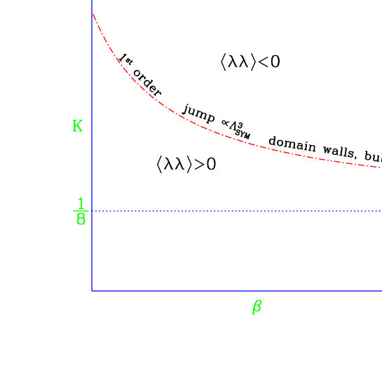
Figure 5: Expected phase structure of Yang-Mills theory with a Majorana fermion in adjoint representation in the ($\beta,K$)-plane. The dashed-dotted line $K=K_{cr}(\beta)$ is a first order phase transition (or cross-over) at zero gaugino mass.

The DESY-Münster Collaboration performed a first lattice investigation of gaugino condensation in SYM theory with SU(2) gauge group [52]. The distribution of $\langle\lambda\lambda\rangle$ has been studied for fixed gauge coupling $\beta=2.3$ as a function of the hopping parameter $K$, which determines the bare gaugino mass, on $6^{3}\cdot 12$ lattice.

A first order phase transition shows up on small to moderately large lattices as metastability expressed by a two-peak structure in the distribution of the gaugino condensate. By tuning $K$ one should be able to achieve that the two peaks are equal (in height or area). This is a possible definition of the phase transition point in finite volumes. By increasing the volume the tunneling between the two ground states becomes less and less probable and at some point practically impossible.

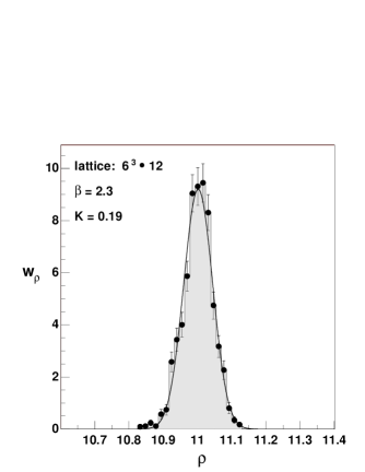
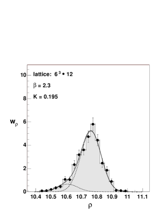
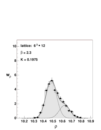
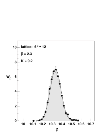
Figure 6: The probability distributions of the gaugino condensate $\rho\equiv\langle\lambda\lambda\rangle$ for different hopping parameters at $\beta=2.3$ on $6^{3}\cdot 12$ lattice. The dased lines show the Gaussian components.

The observed distributions are shown in figure 6. One can see that the distributions cannot always be described by a single Gaussian which would correspond to a single phase. Parameters of possible fits are collected in table 1.

Table 1: Fit parameters of the distributions of gaugino condensate corresponding to figure 6. The weight of the first peak is $p_{1}$, the mean values are $\mu_{1,2}$ and the common width of the Gaussians is $\sigma$. The statistical errors in last digits are given in parentheses.

$K$	$p_{1}$	$\mu_{1}$	$\mu_{2}$	$\sigma$	$\chi^{2}/d.o.f.$
0.19	1.0	11.0023(26)	-	0.0423(16)	27.9/20
0.1925	1.0	10.8807(30)	-	0.0524(17)	25.9/20
0.195	0.89(7)	10.762(30)	10.608(30)	0.066(7)	16.5/18
0.196	0.35(7)	10.722(11)	10.588(11)	0.073(3)	5.7/18
0.1975	0.26(5)	10.626(17)	10.484(17)	0.056(4)	19.5/18
0.2	0.0	-	10.3363(37)	0.0562(18)	21.4/20

As the table shows, in the region $0.195\leq K\leq 0.1975$ only two-Gaussian fits work. Outside this region single Gaussian fits describe the data well. For increasing $K$ (decreasing bare gaugino mass) the weights shift from the Gaussian at larger $\rho\equiv\langle\lambda\lambda\rangle$ to the one with smaller $\rho$, as expected. The two Gaussians represent the contributions of the two phases on this lattice. The position of the phase transition (or cross-over) on the $6^{3}\cdot 12$ lattice is at $K_{0}=0.1955\pm 0.0005$. According to table 1 the jump of the order parameter is $\Delta\rho\equiv\mu_{1}-\mu_{2}\simeq 0.15$.

The two-phase structure can also be searched for in pure gauge field variables as the plaquette or longer Wilson loops. It turns out that the distributions of Wilson loops are rather insensitive. They can be well described by single Gaussians with almost constant variance in the whole range $0.19\leq K\leq 0.2$ [52].

As shown by figure 6 and table 1, on this small lattice the two peaks corresponding to two phases are not well separated. It is possible that at this $\beta$ value there is no genuine first order phase transition at all – only a cross-over. The question of first order phase transition versus cross-over can be decided by studying the volume dependence on larger lattices. After extracting the jump of the gaugino condensate in the large (infinite) volume limit one has to study its behaviour in the continuum limit $\beta\to\infty$ along the line $K_{cr}(\beta)$ in figure 5. The renormalized gaugino condensate can be obtained in the continuum limit by additive and multiplicative renormalizations:

$$\langle\bar{\lambda}_{x}\lambda_{x}\rangle_{R(\mu)}=Z(a\mu)\left[\langle\bar{\lambda}_{x}\lambda_{x}\rangle-b_{0}(a\mu)\right]\ .$$ (80)

The presence of the additive shift in the gaugino condensate $b_{0}(a\mu)$ implies that the value of its jump at $m_{\tilde{g}}=0$ is easier available than the value itself.

The renormalization factor $Z$ in (80) is expected to be of order ${\cal O}(1)$ at bare parameter values which can be reached by numerical simulations. For obtaining it one can use non-perturbative renormalization schemes (for a recent review see [53]). Performing perturbative calculations in lattice regularization can also give useful information [54, 55].

5 Confinement and particle spectrum

5.1 Fundamental static potential

The potential between static colour sources in gauge field theory is a physically interesting quantity because it is characteristic for the dynamics of the gauge field. The external static soursec can be put in any representation of the gauge group. If the sources are in the fundamental representation we have to do with the fundamental static potential between static quarks.

For a model containing dynamical matter fields in the fundamental representation, as is the case for QCD, the charge of static quarks will be screened. The potential then approaches a constant at large distances. The string tension $\sigma$, which is the asymptotic slope of the potential for large distances, vanishes accordingly. On the other hand, if only matter fields in the adjoint representation of the gauge group are present, as in the case of N=1 SYM theory, confinement of static quarks and a positive $\sigma$ are expected.

The DESY-Münster Collaboration has determined the static quark potential and the string tension for N=1 SUSY Yang-Mills theory with gauge group SU(2) in Monte Carlo simulations [42]. The starting point of numerical work are expectation values of rectangular Wilson loops $\langle W(R,T)\rangle$ of spatial length $R$ and time length $T$. From the Wilson loops the potential can be found via

$$V(R)=\lim_{T\to\infty}V(R,T)\ ,$$ (81)

where

$$V(R,T)=\log\langle W(R,T)\rangle-\log\langle W(R,T+1)\rangle\ .$$ (82)

The potential $V(R)$ is obtained through a fit of the form

$$V(R,T)=V(R)+c_{1}(R)e^{-c_{2}(R)T}.$$ (83)

The string tension $\sigma$ is finally obtained by fitting the potential according to

$$V(R)=V_{0}-\frac{\alpha}{R}+\sigma R.$$ (84)

An example of the static quark potential on $12^{3}\cdot 24$ lattice at $\beta=2.3$, $K=0.1925$ is shown in figure 7.

Figure 7: The static quark potential $V(R)$ on a $12^{3}\cdot 24$ lattice at $\beta=2.3$, $K=0.1925$. The line is a fit with a Coulomb plus a linear term, fitted over the range $1\leq R\leq 6$.

A collection of the results for the string tension on lattices with spatial extension $L$ is:

$$a\sqrt{\sigma} = 0.22(1)\hskip 14.22636pt\mbox{for}\ K=0.1900,\ L=8,$$

$$a\sqrt{\sigma} = 0.21(1)\hskip 14.22636pt\mbox{for}\ K=0.1925,\ L=8,$$

$$a\sqrt{\sigma} = 0.17(1)\hskip 14.22636pt\mbox{for}\ K=0.1925,\ L=12.$$ (85)

The string tension in lattice units is decreasing when the critical line is approached, as it should be. This is mainly caused by the renormalization of the gauge coupling due to virtual gluino loop effects which are manifested by decreasing lattice spacing $a$. From a comparison of the $L=8$ and $L=12$ results one sees that finite size effects still appear to be sizable. This has to be expected because we have for the spatial lattice extension $L=12a$ the result $L\sqrt{\sigma}\simeq 2.1$. In QCD with $\sqrt{\sigma}\simeq 0.45\,GeV$ this would correspond to $L\simeq 1\,fm$. Although we are dealing with a different theory where finite size effects as a function of $L\sqrt{\sigma}$ are different, for a first orientation this estimate should be good enough.

For the ratio of the scalar glueball mass $m(0^{+})$, to be discussed below, and the square root of the string tension the results are:

$$m(0^{+})/\sqrt{\sigma} = 3.4(7)\hskip 8.53581pt\mbox{for}\ K=0.1900,\ L=8,$$

$$m(0^{+})/\sqrt{\sigma} = 3.0(4)\hskip 8.53581pt\mbox{for}\ K=0.1925,\ L=8,$$

$$m(0^{+})/\sqrt{\sigma} = 3.1(7)\hskip 8.53581pt\mbox{for}\ K=0.1925,\ L=12.$$ (86)

The uncertainties are not very small, but the numbers are consistent with a constant independent of $K$ in this range.

5.2 Supersymmetry multiplets?

The non-vanishing string tension implies that the Yang-Mills theory with gluinos is confining. Therefore the asymptotic states are colour singlets, similarly to hadrons in QCD. The structure of the light hadron spectrum is closest to the (theoretical) case of QCD with a single flavour of quarks where the chiral symmetry is broken by the anomaly.

Since both gluons and gluinos transform according to the adjoint (for SU(2) gauge group triplet) representation of the colour group, one can construct colour singlet interpolating fields from any number of gluons and gluinos if their total number is at least two. Experience in QCD suggests that the lightest states can be well represented by interpolating fields built out of a small number of constituents. Simple examples are the glueballs known from pure Yang-Mills theory and gluinoballs which are composite states made out of gluinos. Mixed gluino-glueball states can be composed of any number of gluons and any number of gluinos, in the simplest case just one of both.

In general, one has to keep in mind that the classification of states by some interpolating fields has only a limited validity, because this is a strongly interacting theory where many interpolating fields can have important projections on the same state. Taking just the simplest colour singlets can, however, give a good qualitative description.

In the supersymmetric limit at zero gluino mass $m_{\tilde{g}}=0$ the hadronic states should occur in supermultiplets. This restricts the choice of simple interpolating field combinations and leads to low energy effective actions in terms of them [18, 21]. For non-zero gluino mass the supersymmetry is softly broken and the hadron masses are supposed to be analytic functions of $m_{\tilde{g}}$. The linear terms of a Taylor expansion in $m_{\tilde{g}}$ are often determined by the symmetries of the low energy effective actions [20].

The effective action of Veneziano and Yankielowicz [18] in eq. (23) describes a chiral supermultiplet consisting of the $0^{-}$ gluinoball $\tilde{\eta}$, the $0^{+}$ gluinoball $\tilde{f}_{0}$ and a spin $\frac{1}{2}$ gluino-glueball $\tilde{\chi}$. There is, however, no a priori reason to assume that glueball states are heavier than the members of this supermultiplet. Therefore Farrar, Gabadadze and Schwetz [21] proposed an effective action which includes an additional chiral supermultiplet. This consists of a $0^{+}$ glueball, a $0^{-}$ glueball and another gluino-glueball. The effective action allows mass mixing between the members of the two supermultiplets.

The spectrum of SYM theory with SU(2) gauge group has been studied in numerical simulations by the DESY-Münster Collaboration [42, 56, 57]. The glueball states as well as the methods to compute their masses in numerical Monte Carlo simulations are well known from pure gauge theory (see [23]). The obtained masses for the $0^{+}$ glueball in lattice units are

$$am(0^{+}) = 0.95(10)\hskip 8.53581pt\mbox{for}\ K=0.1800,\ L=6,$$

$$am(0^{+}) = 0.85(6)\hskip 14.22636pt\mbox{for}\ K=0.1850,\ L=6,$$

$$am(0^{+}) = 0.75(6)\hskip 14.22636pt\mbox{for}\ K=0.1900,\ L=8,$$

$$am(0^{+}) = 0.63(5)\hskip 14.22636pt\mbox{for}\ K=0.1925,\ L=8,$$

$$am(0^{+}) = 0.53(10)\hskip 8.53581pt\mbox{for}\ K=0.1925,\ L=12.$$ (87)

As before, $L$ denotes the spatial extension of the lattice. (The time extension has always been $T=2L$.)

In addition to the $J^{P}=0^{+}$ glueball one can also search for the pseudoscalar $0^{-}$ glueball. The masses in lattice units turned out to be

$$am(0^{-}) = 1.5(3)\hskip 19.91692pt\mbox{for}\ K=0.1850,\ L=6,$$

$$am(0^{-}) = 1.45(10)\hskip 8.53581pt\mbox{for}\ K=0.1900,\ L=6,$$

$$am(0^{-}) = 1.3(1)\hskip 19.91692pt\mbox{for}\ K=0.1925,\ L=6,$$

$$am(0^{-}) = 1.1(1)\hskip 19.91692pt\mbox{for}\ K=0.1925,\ L=8.$$ (88)

The pseudoscalar glueball appears to be roughly twice as heavy as the scalar one. This is similar to pure SU(2) gauge theory, where $m(0^{-})/m(0^{+})=1.8(2)$ [23].

As discussed above, besides the glueballs made out of gluons one also has to consider gluinoballs. Examples of simple colourless composite fields can be constructed from two gluino fields: $\overline{\lambda}_{x}\gamma_{5}\lambda_{x}$ and $\overline{\lambda}_{x}\lambda_{x}$. These correspond to the gluinoball states mentioned above: $\tilde{\eta}$ and $\tilde{f}_{0}$, respectively, which are described by the effective action (23).

The masses of $\tilde{\eta}$ and $\tilde{f}_{0}$ can be extracted from correlation functions as

$$\Gamma_{\tilde{g}\tilde{g}}(x,y)=\langle{\rm Tr_{sc}}\,\{\Gamma Q^{-1}_{xx}\}{\rm Tr_{sc}}\,\{\Gamma Q^{-1}_{yy}\}-2\,{\rm Tr_{sc}}\,\{\Gamma Q^{-1}_{xy}\Gamma Q^{-1}_{yx}\}\rangle\ ,$$ (89)

where $\Gamma\in\{1,\gamma_{5}\}$ and $Q^{-1}$ is the gluino propagator. Note that the factor of two is originating from the Majorana character of the gluinos. In analogy with the flavour singlet meson in QCD the correlator in (89) consists of a connected and a disconnected part. The disconnected part can be calculated using the volume source technique [58].

In case of the $\tilde{f}_{0}$ particle the disconnected and the connected parts are of the same order of magnitude whereas $\tilde{\eta}$ is dominated by the connected part. The disconnected part has a much worse signal to noise ratio than the connected one. This leads to a larger error on the $\tilde{f}_{0}$ mass as compared to the $\tilde{\eta}$ mass.

In the low energy effective action of Farrar, Gabadadze and Schwetz [21] there is a possible non-zero mixing between the states in two light supermultiplets. In particular there can be mixing of the $\tilde{f}_{0}$ gluinoball and the $0^{+}$ glueball which have identical quantum numbers. The numerical simulations show that this mixing is small [42, 57].

The low mass supermultiplets containing $J^{P}=0^{-},0^{+}$ states have to be completed by a spin $\frac{1}{2}$ state. The corresponding composite fields can constructed from the gluino field and the field strength tensor of gluons. The simplest example is [27, 57]:

$$\Phi\equiv\sigma_{\mu\nu}\,{\rm Tr\,}\left[F_{\mu\nu}\lambda\right]\ .$$ (90)

On the lattice one has to use, of course, an appropriate construction for $F_{\mu\nu}$ out of the link variables $U_{x\mu}$. Composite fields with the same quantum numbers can also be built up from three gluino fields [56, 57]. A summary of the results of the DESY-Münster Collaboration about the spectrum of light composite states is shown in figure 8.

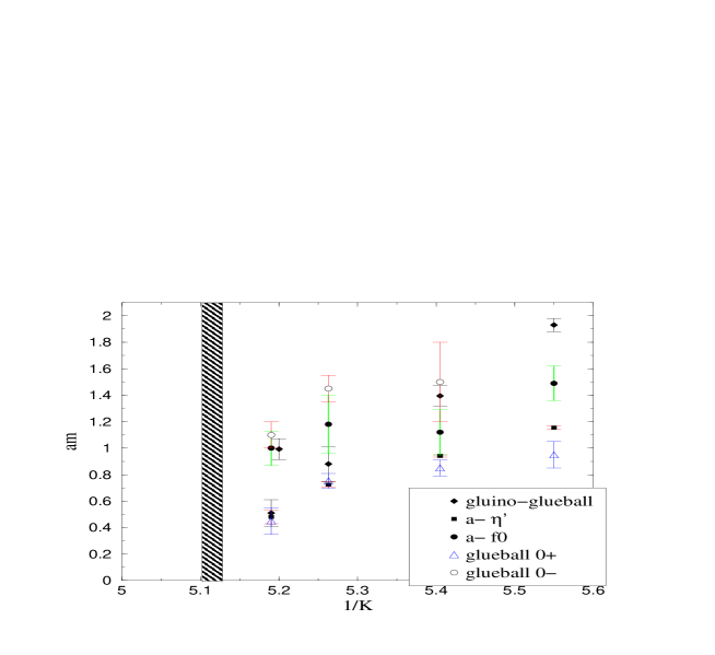
Figure 8: The lightest bound state masses in lattice units as function of the bare gluino mass parameter $1/K$ for fixed $\beta=2.3$. The shaded area at $K=0.1955(5)$ is where zero gluino mass and supersymmetry are expected. In this figure the notations of [42, 56, 57] are used: $a$-$\eta^{\prime}\equiv\tilde{\eta}$ and $a$-$f_{0}\equiv\tilde{f}_{0}$.

As the figure shows, the low mass states appear to build two groups which may correspond to the effective action [21]. For a firm conclusion more numerical work is needed in larger volumes and for several values of the gauge coupling $\beta$ allowing for a continuum extrapolation.

6 Supersymmetric Ward-Takahashi identities

An important feature of lattice regularization is that some symmetries are broken for non-zero lattice spacing and are expected to be recovered in the continuum limit. The details of the lattice formulation, which may also influence the degree of symmetry breaking, are not relevant in the continuum limit because of the universality of critical points. A basic set of symmetries broken by the lattice and restored in the continuum limit is the (Euclidean) Lorentz symmetry including rotations and translations. It is clear that on any regular lattice these symmetries are always broken. Internal symmetries as, for instance, global chiral symmetry are sometimes broken sometimes conserved on the lattice, depending on the actual formulation. From the point of view of symmetry realization supersymmetry is expected to behave similarly to the Lorentz symmetry: at finite lattice spacing it is broken but it becomes restored in the continuum limit. This similarity is quite natural since there is an intimate relation of supersymmetry to the Lorentz symmetries of space-time shown, for instance, by the fact that the anticommutators of the supersymmetry charges give translations.

In the framework of quantum field theory the symmetries can be exploited by the corresponding Ward-Takahashi (WT) identities. Well studied examples are the global axial (chiral) symmetries in lattice QCD [59]. In case of SYM theory this way of realizing supersymmetry has been first considered by Curci and Veneziano [35]. At zero gaugino mass both supersymmetry and anomalous chiral symmetry has to be manifested in the corresponding WT identities.

Before going to the lattice formulation let us describe the WT identities of supersymmetry in the continuum at a somewhat formal, non-rigorous level (for a more rigorous treatment see [4]). The corresponding supercurrent $S_{\mu}$ has been introduced in (5):

$$S_{\mu}(x)\equiv-F^{a}_{\rho\tau}(x)\sigma_{\rho\tau}\gamma_{\mu}\lambda^{a}(x)=-\frac{2i}{g}\sigma_{\rho\tau}\gamma_{\mu}\,{\rm Tr\,}\left(F_{\rho\tau}(x)\lambda(x)\right)\ ,$$ (91)

where the field strength tensor matrix $F_{\mu\nu}(x)$ is defined in (7) and the gaugino field matrix is $\lambda(x)\equiv\lambda^{a}(x)T_{a}$. Since the regularization breaks supersymmetry the simple conservation low $\partial_{\mu}S_{\mu}(x)=0$ can only be recovered in the process of renormalization if the possible operator mixings are properly taken into account. The analysis of the operator mixings [49] leads to the following conjecture about the form of SUSY-WT identities:

$$\langle Z_{S}\partial_{\mu}S_{\mu}(x){\cal O}(y)+Z_{T}\partial_{\mu}T_{\mu}(x){\cal O}(y)\rangle=(m_{0}-\bar{m})\langle D_{S}(x){\cal O}(y)\rangle\ .$$ (92)

Here ${\cal O}(y)$ is any gauge invariant local operator at point $y$ and $T_{\mu}(x)$ is another dimension $\frac{7}{2}$ operator besides $S_{\mu}(x)$, namely

$$T_{\mu}(x)=\frac{2i}{g}\gamma_{\nu}\,{\rm Tr\,}\left(F_{\mu\nu}(x)\lambda(x)\right)\ .$$ (93)

The operator $D_{S}(x)$ appearing on the right hand side of (92) is defined as

$$D_{S}(x)=\frac{2i}{g}\sigma_{\mu\nu}\,{\rm Tr\,}\left(F_{\mu\nu}(x)\lambda(x)\right)\ .$$ (94)

$Z_{S}$ and $Z_{T}$ are multiplicative renormalization factors, $m_{0}$ is the bare gaugino mass and $\bar{m}$ represents the additive renormalization of the bare mass. The form of (92) is valid only for $x\neq y$ because “contact terms” have been omitted. The consequence of (92) is that the (renormalized) gaugino mass vanishes if $m_{0}-\bar{m}=0$ and the renormalized supercurrent can be defined as

$$\hat{S}_{\mu}(x)\equiv Z_{S}S_{\mu}(x)+Z_{T}T_{\mu}(x)\ .$$ (95)

6.1 Lattice formulation

The arguments leading to the SUSY-WT identity (92) can be followed step by step in lattice regularization. First one has to define the supersymmetry transformations. Since SUSY is broken on the lattice the lattice action will not be invariant with respect to these transformations. There is a freedom in the definition which is only restricted by the requirement that in the continuum limit the infinitesimal transformations in (3) have to be reproduced. The supersymmetry breaking terms, which should vanish as ${\cal O}(a)$ in the continuum limit $a\to 0$, can be minimized by an appropriate choice of the irrelevant parts. An important requirement is to maintain as many discrete lattice symmetries as possible. In particular the parity ${\cal P}$, time reversal ${\cal T}$ and charge conjugation ${\cal C}$ transformations should commute with the lattice SUSY transformations.

A simple choice fulfilling these requirement has been introduced in [54]. For these definitions let us change the conventions in the lattice action for gauginos (43) by changing the normalization of the gaugino field according to

$$\lambda_{x}\to\sqrt{m_{0}+4}\;\lambda_{x}$$ (96)

and introduce the bare lattice mass $m_{0}$ by

$$m_{0}\equiv\frac{1}{2K}-4\ ,\hskip 30.00005ptK=\frac{1}{2(m_{0}+4)}\ .$$ (97)

Using the gaugino field matrix $\lambda_{x}\equiv\lambda^{a}_{x}T_{a}$ we have instead of (43) the fermionic action

$$S_{f}=\sum_{x}{\rm Tr\,}\raisebox{-1.29167pt}{\mbox{\LARGE$\left\{\right.$}}(m_{0}+4)\overline{\lambda}_{x}\lambda_{x}-\frac{1}{2}\sum_{\mu=1}^{4}\left[\overline{\lambda}_{x+\hat{\mu}}U_{x\mu}(1+\gamma_{\mu})\lambda_{x}U^{\dagger}_{x\mu}+\overline{\lambda}_{x}U^{\dagger}_{x\mu}(1-\gamma_{\mu})\lambda_{x+\hat{\mu}}U_{x\mu}\right]\raisebox{-1.29167pt}{\mbox{\LARGE$\left.\right\}$}}\ .$$ (98)

(Note that compared to ref. [54] $U_{x\mu}$ is replaced here by $U^{\dagger}_{x\mu}$.) This notation is close to the continuum conventions whereas (43) is practical for numerical simulations. For the definition of the SUSY transformations we need an appropriately defined field strength tensor on the lattice which we denote by $P_{\mu\nu}(x)$:

$$P_{\mu\nu}(x) \equiv \frac{1}{8ig}\sum_{i=1}^{4}\left[U_{i\mu\nu}(x)-U^{\dagger}_{i\mu\nu}(x)\right]\ ,$$

$$U_{1\mu\nu}(x) \equiv U^{\dagger}_{x\nu}U^{\dagger}_{x+\hat{\nu},\mu}U_{x+\hat{\mu},\nu}U_{x\mu}\ ,$$

$$U_{2\mu\nu}(x) \equiv U^{\dagger}_{x\mu}U_{x-\hat{\nu}+\hat{\mu},\nu}U_{x-\hat{\nu},\mu}U^{\dagger}_{x-\hat{\nu},\nu}\ ,$$

$$U_{3\mu\nu}(x) \equiv U_{x-\hat{\nu},\nu}U_{x-\hat{\nu}-\hat{\mu},\mu}U^{\dagger}_{x-\hat{\nu}-\hat{\mu},\nu}U^{\dagger}_{x-\hat{\mu},\mu}\ ,$$

$$U_{4\mu\nu}(x) \equiv U_{x-\hat{\mu},\mu}U^{\dagger}_{x-\hat{\mu},\nu}U^{\dagger}_{x+\hat{\nu}-\hat{\mu},\mu}U_{x\nu}\ .$$ (99)

This transforms under parity and time reversal in the same way as $F_{\mu\nu}$ does in the continuum. Using $P_{\mu\nu}(x)$ one can define the infinitesimal SUSY transformations on the lattice by

$$\delta_{\xi}U_{x\mu} = -\frac{ig}{2}\left[\overline{\xi}\gamma_{\mu}U_{x\mu}\lambda_{x}+\overline{\xi}\gamma_{\mu}\lambda_{x+\hat{\mu}}U_{x\mu}\right]\ ,$$

$$\delta_{\xi}U^{\dagger}_{x\mu} = \frac{ig}{2}\left[\overline{\xi}\gamma_{\mu}\lambda_{x}U^{\dagger}_{x\mu}+\overline{\xi}\gamma_{\mu}U^{\dagger}_{x\mu}\lambda_{x+\hat{\mu}}\right]\ ,$$

$$\delta_{\xi}\lambda_{x} = \frac{1}{2}\sigma_{\mu\nu}\xi P_{\mu\nu}(x)\ ,$$

$$\delta_{\xi}\overline{\lambda}_{x} = -\frac{1}{2}\overline{\xi}\sigma_{\mu\nu}P_{\mu\nu}(x)\ .$$ (100)

Here $\xi$ and $\overline{\xi}$ are Grassmannian parameters satisfying a Majorana condition like (2).

After defining the lattice SUSY transformations (6.1) one can derive the SUSY WT-identities by a standard procedure [59, 26]. The corresponding lattice supercurrent $S_{\mu}(x)$ can be identified as

$$S_{\mu}(x)=-\frac{1}{2}\sum_{\rho\sigma}\sigma_{\rho\sigma}\gamma_{\mu}{\rm\,Tr\,}\left[P_{\rho\sigma}(x)U^{\dagger}_{x\mu}\lambda_{x+\hat{\mu}}U_{x\mu}+P_{\rho\sigma}(x+\hat{\mu})U_{x\mu}\lambda_{x}U^{\dagger}_{x\mu}\right]\ .$$ (101)

The spinorial density multiplying the gaugino mass turns out to be

$$D_{S}(x)=\sum_{\rho\sigma}\sigma_{\rho\sigma}{\rm\,Tr\,}\left[P_{\rho\sigma}(x)\lambda_{x}\right]\ .$$ (102)

The other supercurrent $T_{\mu}(x)$ which is mixed to $S_{\mu}(x)$ can be defined as

$$T_{\mu}(x)=\sum_{\nu}\gamma_{\nu}{\rm\,Tr\,}\left[P_{\mu\nu}(x)U^{\dagger}_{x\mu}\lambda_{x+\hat{\mu}}U_{x\mu}+P_{\mu\nu}(x+\hat{\mu})U_{x\mu}\lambda_{x}U^{\dagger}_{x\mu}\right]\ .$$ (103)

In the continuum limit, apart from differences in normalization conventions, these supercurrents go over to their continuum conterparts in (91)-(94).

Using these definitions the SUSY WT-identity can be written as [35, 27, 54]:

$$Z_{S}\langle\nabla^{b}_{\mu}S_{\mu}(x){\cal O}(y)\rangle+Z_{T}\langle\nabla^{b}_{\mu}T_{\mu}(x){\cal O}(y)\rangle=(m_{0}-\bar{m})\langle D_{S}(x){\cal O}(y)\rangle+{\cal O}(a)\ .$$ (104)

Here the lattice (backward) derivative is defined as $\nabla^{b}_{\mu}f(x)\equiv f(x)-f(x-\hat{\mu})$. The gauge invariant function ${\cal O}(y)$ at point $y$ is assumed to be sufficiently far away from $x$ in such a way that no common points with the expressions defined at $x$ occur. In this way additional contact terms are avoided.

The SUSY WT-identity as it stands in (104) is only valid for gauge invariant functions ${\cal O}(y)$ of lattice fields. In case of gauge non-invariance several additional terms appear. Examples of such anomalous terms emerge, for instance, in lattice perturbation theory calculations [54, 55]. The reason behind these complications is the conflict of gauge fixing with supersymmetry.

As already remarked above, the form of the lattice currents in (101)-(103) is not unique because terms of order ${\cal O}(a)$ can be added. Locality and simplicity of the expressions is always welcome. This leads to the alternative definitions of the “local” supercurrents

$$S^{l}_{\mu}(x)=-\sum_{\rho\sigma}\sigma_{\rho\sigma}\gamma_{\mu}{\rm\,Tr\,}\left[P_{\rho\sigma}(x)\lambda_{x}\right]$$ (105)

and

$$T^{l}_{\mu}(x)=2\sum_{\nu}\gamma_{\nu}{\rm\,Tr\,}\left[P_{\mu\nu}(x)\lambda_{x}\right]\ .$$ (106)

In contrast to these we can call the supercurrents in (101) and (103) as “point-split”:

$$S^{ps}_{\mu}(x)\equiv S_{\mu}(x)\ ,\hskip 30.00005ptT^{ps}_{\mu}(x)\equiv T_{\mu}(x)\ .$$ (107)

In addition to the ambiguity of supercurrents the lattice approximation of the derivatives can also be varied. For instance, for the local supercurrents in (105) and (106) the backward difference $\nabla^{b}\mu$ may be replaced by a “symmetric difference” $\nabla^{s}_{\mu}f(x)\equiv\frac{1}{2}(f(x+\hat{\mu})-f(x-\hat{\mu}))$. All these variations are irrelevant in the continuum limit but for non-zero lattice spacing $a\neq 0$ the ${\cal O}(a)$ lattice artefacts in (104) can be rather different.

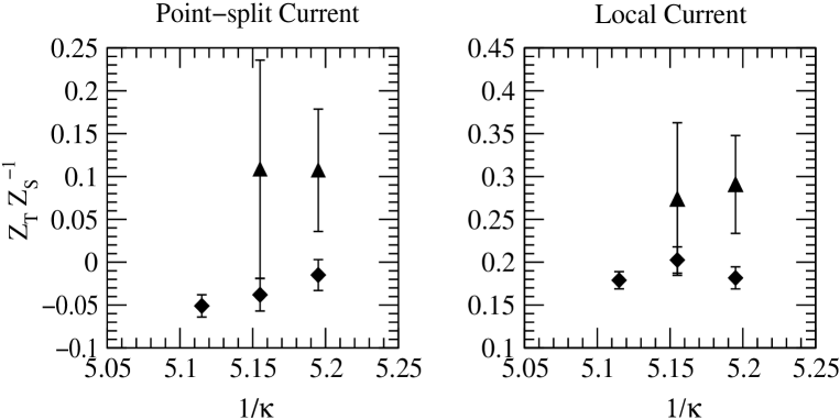
Figure 9: Results for the supercurrent renormalization factors from [49]. On the horizontal axis the inverse hopping parameter values are shown ($1/\kappa\equiv 1/K$).

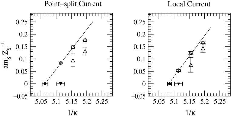
Figure 10: Results for the renormalized gaugino mass from [49]. On the horizontal axis the invers hopping parameter values are shown ($1/\kappa\equiv 1/K$). The dashed lines are linear extrapolations for vanishing gaugino mass.

6.2 Numerical results

The DESY-Münster-Roma Collaboration studied the SUSY WT-identities in numerical simulations [48, 49]. Omitting ${\cal O}(a)$ terms and dividing by $Z_{S}$ the SUSY WT-identity in (104) can be brought to the form [27]

$$\langle\nabla^{b}_{\mu}S_{\mu}(x){\cal O}(y)\rangle+\frac{Z_{T}}{Z_{S}}\langle\nabla^{b}_{\mu}T_{\mu}(x){\cal O}(y)\rangle=\frac{(m_{0}-\bar{m})}{Z_{S}}\langle D_{S}(x){\cal O}(y)\rangle\ .$$ (108)

This has to be valid for every gauge invariant function ${\cal O}(y)$ which is defined in a point $y$ in such a way that there are no common points with the functions defined at $x$. Considering (108) with different ${\cal O}(y)$ a system of linear equations is obtained for the two unknowns

$$z_{TS}\equiv\frac{Z_{T}}{Z_{S}}\ ,\hskip 30.00005ptz_{MS}\equiv\frac{(m_{0}-\bar{m})}{Z_{S}}\ .$$ (109)

(Note that $z_{MS}$ is proportional to the renormalized gaugino mass $m_{R}\equiv(m_{0}-\bar{m})/Z_{m}$.) Since there are very many different possible ${\cal O}(y)$’s, the expectation that (108) has, in the continuum limit, a unique solution pair $(z_{TS},z_{MS})$ is highly non-trivial. Its numerical investigation can strongly support (or perhaps contradict) our expectations about the realization of supersymmetry in SYM theory.

For obtaining non-zero expectation values the gauge invariant functions ${\cal O}(y)$ appearing in (109) have to be chosen appropriately. Roughly speaking they should have quantum numbers similar to the spinorial density $D_{S}(x)$. The intermediate states with important contributions are composite states of a gluino (= gaugino) and a gluon as, for instance, the gluino-glueball $\tilde{\chi}$ investigated in section 5.2. In order to obtain a good signal to noise ratio one can sum over three $x$-coordinates $(x_{1},x_{2},x_{3})$ keeping the fourth time-coordinate fixed. This projects out intermediate states with zero spatial momentum. One can also apply optimized smearing techniques in the timeslice containing $y$ similarly to correlators for obtaining the masses of gluino-glueballs.

Table 2: The values of $r_{0}/a$ for the sets of configurations considered in [49]. The ratio $L/r_{0}$ is also shown, where $L$ is the spatial lattice size.

$\kappa$	$r_{0}/a$	$L/r_{0}$
0.1925	6.71(19)	1.79(5)
0.194	7.37(30)	1.63(7)
0.1955	7.98(48)	1.50(9)

The numerical simulations of the DESY-Münster-Roma Collaboration [49] has been performed on a $12^{3}\cdot 24$ lattice at $\beta=2.3$ for three different values of the bare gaugino mass given by $K=0.1925,\;0.1940,\;0.1950$. These parameters are well suited for a first study because they are reasonably close to the continuum limit and since the WT-identities hold in any volume no finite volume effects are disturbing. The values of the scale parameter $r_{0}$ [60], which give information about the physical volume size, are shown in table 2. A summary of the resulting fits to $z_{TS}$ and $z_{MS}$ is contained in figures 9 and 10. (For more details see [49].)

The renormalization factors $Z_{S}$ and $Z_{T}$ depend on the definition of the lattice supercurrents. As figure 9 shows, the admixture of $T_{\mu}(x)$ is negligible for the point-split supercurrent $S^{ps}_{\mu}(x)$ but non-zero for the local supercurrent $S^{l}_{\mu}(x)$. $z_{TS}$ is within errors independent of the bare mass given by $K$. $z_{MS}$ is proportional to the renormalized mass and tends to zero if $K$ approaches the critical value $K_{cr}$.

These results are consistent with expectations, in particular with the realization of supersymmetry in a Yang-Mills theory with massless Majorana fermion in the adjoint representation. For a stronger conclusion the continuum limit $\beta\to\infty$ has to be investigated in future simulations.

7 Outlook

The numerical Monte Carlo simulation of supersymmetric Yang-Mills theory is feasible with presently available computational resources and with known algorithms. The total computational effort of the DESY-Münster-Roma Collaboration has been of the order of 10 Gflops $\cdot$ year $\simeq 3\cdot 10^{17}$ floating point operations. This is much less than the amount of computer time devoted up to now to QCD. In fact, to simulate SYM theory is substantially easier than QCD because the “flavour number” of fermions $N_{f}=\frac{1}{2}$ is smaller. In addition, in contrast to QCD, in SYM there are no almost massless pseudoscalar mesons expected. The easiness and the considerable theoretical interest make the Monte Carlo simulation of SYM theory a promising future subject.

The next steps in improving the present simulations are obvious:

• clarification of the nature of the transition at vanishing gaugino mass by studying its behaviour on larger lattice volumes;

• investigation of the spectrum of bound states in supermultiplets in sufficiently large volumes and closer to the continuum limit;

• study of the continuum limit of the supersymmetric Ward-Takahashi identities.

Once these basic questions are sufficiently clarified one can certainly find other more detailed questions which will help understanding many aspects of the dynamics of supersymmetric gauge field theories.

Acknowledgements

The numerical simulation results summarized in this review have been obtained due to the enthusiastic work done by the members of the DESY-Münster-Roma Collaboration. I thank them for valuable discussions and comments. The Monte Carlo runs have been performed on the CRAY-T3E supercomputers at NIC Jülich. It is a pleasure to thank the staff at NIC for their kind support.

References

- [1] N. Seiberg and E. Witten, Nucl. Phys. B426, 19 (1994); ERRATUM ibid. B430, 485 (1994).
-
[2]
H. Nicolai,
Nucl. Phys. B140, 294 (1978);
P. van Nieuwenhuizen, A. Waldron, Phys. Lett. B389, 29 (1996). -
[3]
J. Bagger, J. Wess,
Supersymmetry and Supergravity,
Princeton University Press, 1983;
P. Fayet, S. Ferrara, Phys. Rep. 32, 249 (1977);
M.F. Sohnius, Phys. Rep. 128, 39 (1985). - [4] C. Rupp, K. Sibold, hep-th/0101165.
- [5] A. Feo et al. (DESY-Münster Collaboration), Nucl. Phys. Proc. Suppl. 83, 661 (2000).
- [6] I. Affleck, M. Dine, N. Seiberg, Phys. Rev. Lett. 51, 1026 (1983); Nucl. Phys. B241, 493 (1984).
- [7] V.A. Novikov, M.A. Shifman, A.I. Vainshtein, V.I. Zakharov, Nucl. Phys. B260, 157 (1985).
- [8] M.A. Shifman, A.I. Vainshtein, Nucl. Phys. B296, 445 (1988).
- [9] D. Finnell, P. Pouliot, Nucl. Phys. B453, 225 (1995).
- [10] V.A. Novikov, M.A. Shifman, A.I. Vainshtein, V.I. Zakharov, Nucl. Phys. B229, 407 (1983).
- [11] G.C. Rossi, G. Veneziano, Phys. Lett. B138, 195 (1984).
- [12] D. Amati, G.C. Rossi, G. Veneziano, Nucl. Phys. B249, 1 (1985).
- [13] D. Amati, K. Konishi, Y. Meurice, G.C. Rossi,G. Veneziano, Phys. Rep. 162, 169 (1988).
- [14] T.J. Hollowood, V.V. Khoze, W. Lee, M.P. Mattis, Nucl. Phys. B570, 241 (2000).
- [15] A. Kovner, M. Shifman, Phys. Rev. D56, 2396 (1997).
- [16] P. Weisz, Phys. Lett. 100B, 331 (1981) and private communication.
- [17] E. Witten, Nucl. Phys. B202, 253 (1982).
- [18] G. Veneziano, S. Yankielowicz, Phys. Lett. B113, 231 (1982).
- [19] S. Ferrara, B. Zumino, Nucl. Phys. B87 207 (1975).
- [20] N. Evans, S.D.H. Hsu, M. Schwetz, hep-th/9707260.
- [21] G.R. Farrar, G. Gabadadze, M. Schwetz, Phys. Rev. D60, 035002 (1999).
- [22] A. Kovner, M. Shifman, A. Smilga, Phys. Rev. D56, 7978 (1997).
-
[23]
C. Michael, M. Teper,
Phys. Lett. B199, 95 (1987);
H. Chen, J. Sexton, A. Vaccarino, D. Weingarten, Nucl. Phys. Proc. Suppl. 34, 357 (1994);
M.J. Teper, in Confinement, Duality and Non-Perturbative Aspects of QCD, NATO Advanced Study Institute, Cambridge 1997 and hep-lat/9711011. - [24] I. Jack, D.R.T. Jones, in Perspectives on supersymmetry, ed. G.L. Kane; hep-ph/9705417.
- [25] A. Casher, Y. Shamir, hep-th/9908074.
- [26] I. Montvay, G. Münster, Quantum Fields on a Lattice, Cambridge University Press, 1994.
- [27] A. Donini, M. Guagnelli, P. Hernandez, A. Vladikas, Nucl. Phys. B523, 529 (1998).
- [28] W. Bietenholz, Mod. Phys. Lett. A14, 51 (1999).
- [29] S. Catterall, S. Karamov, hep-lat/010071.
- [30] D.B. Kaplan, M. Schmaltz, Chin. J. Phys. 38, 543 (2000).
- [31] H. Neuberger, Phys. Rev. D57, 5417 (1998).
- [32] T. Hotta, T. Izubuchi, J. Nishimura, Mod. Phys. Lett. A13, 1667 (1998).
- [33] P.H. Ginsparg, K.G. Wilson, Phys. Rev. D25, 2649 (1982).
- [34] G.T. Fleming, J.B. Kogut, P.M. Vranas, Phys. Rev. D64, 034510 (2001).
- [35] G. Curci and G. Veneziano, Nucl. Phys. B292, 555 (1987).
- [36] S. Gottlieb, W. Liu, D. Toussaint, R.L. Renken, R.L. Sugar, Phys. Rev. D35, 2531 (1987).
- [37] I. Montvay, Nucl. Phys. B466, 259 (1996).
- [38] M. Lüscher, Nucl. Phys. B418, 637 (1994).
- [39] H. Neuberger, Phys. Rev. Lett. 81, 4060 (1998).
- [40] A. Borici, Ph. de Forcrand, Nucl. Phys. B454, 645 (1995).
- [41] R. Frezzotti and K. Jansen, Phys. Lett. B402, 328 (1997).
- [42] I. Campos et al. (DESY-Münster Collaboration), Eur. Phys. J. C11, 507 (1999).
- [43] I. Montvay, Comput. Phys. Commun. 109, 144 (1998); and in Numerical challenges in lattice quantum chromodynamics, Wuppertal 1999, Springer 2000, p. 153; hep-lat/9911014.
- [44] I. Montvay, hep-lat/0111015.
- [45] N. Bourbaki, Algèbre, Chap. IX., Hermann, Paris, 1959.
- [46] R. Kirchner et al. (DESY-Münster Collaboration), Nucl. Phys. Proc. Suppl. 73, 828 (1999).
- [47] R.G. Edwards, U.M. Heller, R. Narayanan, Nucl. Phys. B535, 403 (1998).
- [48] F. Farchioni et al. (DESY-Münster-Roma Collaboration), Nucl. Phys. Proc. Suppl. 94, 787 (2001).
- [49] F. Farchioni et al. (DESY-Münster-Roma Collaboration), hep-lat/0111008.
- [50] S. Hands, I. Montvay, S. Morrison, M. Oevers, L. Scorzato, J. Skullerud, Eur. Phys. J. C17, 285 (2000).
- [51] S. Duane, A.D. Kennedy, B.J. Pendleton, D. Roweth, Phys. Lett. B195, 216 (1987).
- [52] R. Kirchner et al. (DESY-Münster Collaboration), Phys. Lett. B446, 209 (1999).
- [53] S. Sint, Nucl. Phys. Proc. Suppl. 94, 79 (2001).
- [54] Y. Taniguchi, Phys. Rev. D63, 014502 (2001).
- [55] F. Farchioni et al. (DESY-Münster Collaboration), Nucl. Phys. Proc. Suppl. 94, 791 (2001); hep-lat/0110113.
- [56] A. Feo et al. (DESY-Münster Collaboration), Nucl. Phys. Proc. Suppl. 83, 670 (2000).
- [57] R. Kirchner, Ward identities and mass spectrum of N=1 Super Yang-Mills theory on the lattice, PhD Thesis, University Hamburg, 2000.
- [58] Y. Kuramashi, M. Fukugita, H. Mino, M. Okawa, A. Ukawa, Phys. Rev. Lett. 72, 3448 (1994).
- [59] M. Bochicchio, L. Maiani, G. Martinelli, G. Rossi, M. Testa, Nucl. Phys. B262, 331 (1985).
- [60] R. Sommer, Nucl. Phys. B411, 839 (1994).