hep-lat/0112001

ANTISYMMETRIC AND OTHER SUBLEADING CORRECTIONS
TO SCALING IN THE LOCAL POTENTIAL APPROXIMATION

M. M. Tsypin

Department of Physics and Astronomy, Rutgers University,
Piscataway, NJ 08854, USA

and

Institute for Advanced Study, Einstein Drive, Princeton, NJ 08540, USA

Abstract

For systems in the universality class of the three-dimensional Ising model we compute the critical exponents in the local potential approximation (LPA), that is, in the framework of the Wegner-Houghton equation. We are mostly interested in antisymmetric corrections to scaling, which are relatively poorly studied. We find the exponent for the leading antisymmetric correction to scaling $\omega_{A}\approx 1.691$ in the LPA. This high value implies that such corrections cannot explain asymmetries observed in some Monte Carlo simulations.

1 Introduction

This work is devoted to the study of corrections to scaling in the vicinity of the critical point: the endpoint of the line of first order phase transition.

There are many systems that have a critical point belonging to the universality class of the three-dimensional (3D) Ising model. In easy-axis magnetic materials that exhibit a phase transition between paramagnetic and ferromagnetic phases (these systems most directly correspond to the Ising model) the first order phase transition line is in the plane $(T,h)$, where $T$ is the temperature and $h$ is external magnetic field. It is located at $h=0$ and $T<T_{c}$, and ends at the critical point $(T=T_{c},h=0)$.

The system liquid-gas has the line of first order transition, ending at the critical point, in the plane (temperature, pressure). This critical point has been very thoroughly studied. A comprehensive review, as well as additional references, can be found in [1]. Experimental data, theoretical considerations [2, 3] and Monte Carlo simulations of model systems [4] all indicate that it belongs to the 3D Ising model universality class.

The Standard Model of electroweak interactions was shown to have a similar phase transition line in the plane (higgs mass, temperature) [5, 6]. Monte Carlo simulations provide convincing evidence that the endpoint of this line belongs to the 3D Ising universality class [7].

There are strong arguments in favor of a similar first order phase transition line in hot nuclear matter, described by quantum chromodynamics (QCD) at high temperature, in this case in the plane (chemical potential for baryons, temperature) [8, 9]. Its endpoint is conjectured to belong to the 3D Ising universality class [8].

Monte Carlo simulations play an important role in elucidating the critical properties of these systems, especially of more complex ones, such as electroweak matter and nuclear matter at high temperature. These simulations normally have to be performed for systems of relatively small sizes, usually no larger than $64^{3}$ [7] (and often considerably smaller), due to their high complexity and the corresponding high computational load. This means that the system is not very deep into the scaling region (roughly speaking, one cannot reach the correlation length $\xi$ much larger than the system size $L$), and the interpretation of the Monte Carlo data requires proper account for corrections to scaling.

Here we come to the following interesting point. Unlike the Ising model, phase transitions in the liquid-gas system, as well as in electroweak and nuclear matter, do not have the exact global $Z_{2}$ symmetry that corresponds to changing the sign of magnetization in the Ising model, i. e. to simultaneous flipping of all spins. For example, in the Ising model (without external field) the probability distribution for the total magnetization of the system is always perfectly symmetric, despite corrections to scaling, while this is not necessarily so in above-mentioned models. The $Z_{2}$ symmetry is expected to be dynamically restored in the scaling limit [2], but there can be, in addition to the usual corrections to scaling, which are even in the order parameter, also corrections that are odd.

Monte Carlo studies of critical points in such systems, which typically aim at obtaining the linear mapping of the vicinity of the critical point in the plane of parameters of the model onto the corresponding vicinity of the critical point of the 3D Ising model in the $(T,h)$ plane, have to somehow resolve the issue of deviations from the $Z_{2}$ symmetry [4, 7]. Suffice it to say that such mapping requires determination of the magnetization-like ($M$-like) and energy-like ($E$-like) directions in the space of observables, which would be much easier in the presence of $Z_{2}$ symmetry: the requirement that the probability distribution of the $M$-like observable should be symmetric greatly aids the search for the corresponding direction in the space of observables [4].

In practice, the data produced in Monte Carlo simulations demonstrate quite non-negligible deviations from $Z_{2}$ symmetry, and an interesting question is whether these deviations can be attributed to antisymmetric, i. e. $M$-odd, corrections to scaling [7]. Such corrections have attracted much less attention in the literature than the usual ($M$-even) corrections; however, several studies in the framework of the $\epsilon$-expansion [10, 2, 11], as well as renormalization group [12], have been published.

While the usual $M$-even corrections to scaling behave as $L^{-\omega},\ \omega\equiv\Delta/\nu\approx 0.8$, $L$ being the characteristic length in the system, the $M$-odd corrections to scaling are governed by their own exponent $\omega_{A}$ (we prefer this notation [1] to traditional $\omega_{5}$). The $\epsilon$-expansion obtained in [11] reads

$$\omega_{A}=1+{11\over 6}\epsilon-{685\over 324}\epsilon^{2}+{107855+103680\zeta(3)\over 34992}\epsilon^{3}+O(\epsilon^{4}).$$ (1)

At $\epsilon=1$ this series behaves too poorly $(1+1.83-2.11+6.64\ \ldots)$ to get conclusive results; Padé approximants produce the sequence 2.83, 1.85, 2.32 in orders $\epsilon$, $\epsilon^{2}$, $\epsilon^{3}$, respectively, leading to the estimate $\omega_{A}\mathop{\raise 1.29167pt\hbox{$>$\kern-7.5pt\raise-4.73611pt\hbox{$\sim$}}}1.5$ [11]. The renormalization group computation [12] gives $\omega_{A}=2.4(5)$.

These very high values of $\omega_{A}$ imply that $M$-odd corrections to scaling, going as $L^{-\omega_{A}}$, should decay much faster than the leading $M$-even corrections $(L^{-\omega})$, and quickly become negligible when the scaling limit is approached. However, in the Monte Carlo study [7] the asymmetry of the probability distribution of the $M$-like observable at the critical point was found to decay much more slowly with the growing lattice size, more like $L^{-0.5}$.

Before concluding that this observation requires explanation outside the scope of corrections to scaling, one has to be confident that there are indeed no $M$-odd corrections to scaling with small exponents (which could conceivably happen, for example, if existing computations of $\omega_{A}$ somehow missed the leading $M$-odd correction and corresponded instead to a subleading correction). To gain such confidence, we have performed a computation of $M$-odd corrections in the framework of the local potential approximation (LPA), i. e. the Wegner-Houghton equation [13, 14, 15, 16].

The WH equation satisfies our needs nicely, as it reproduces robustly all the relevant features of the theory. In this approximation the critical exponent $\eta$ is zero.

Our study differs from the existing literature on the WH equation [13, 14, 17, 18, 19, 20] in several significant aspects: (1) we are not aware of any previous study of $M$-odd corrections to scaling in the framework of the WH equation, with the exception of unpublished work [21]; (2) we do not rely on avoiding the singularity when solving the WH equation, and thus check whether the large-field domain plays an important role in fixing the values of the critical exponents.

Our main results are as follows. (1) We confirm the absence of $M$-odd corrections to scaling with small exponents. We get the exponent for the leading $M$-odd correction $\omega_{A}\approx 1.691$, which is consistent with [21]. (2) The large-field domain is not important for fixing the critical exponents, at our level of accuracy.

We conclude that the asymmetry observed in [7] is not explainable by $M$-odd corrections to scaling.

The paper is organized as follows. In Sect. 2 we discuss the local potential approximation and the Wegner-Houghton equation. In Sect. 3 we describe our method of finding the fixed point and computing the critical exponents. Sect. 4 contains our numerical results and conclusions.

2 The Wegner-Houghton equation

In this section we remind the reader the structure and the meaning of the WH equation. Accurate derivation can be found in original papers [13, 14] and reviews [15, 16].

The starting point is the description of the system in the vicinity of the critical point by the theory of the 1-component real scalar field $\phi$ with the bare potential $V(\phi)$:

$$\cal{Z} = \int D\phi e^{-S[\phi]},$$ (2)

$$S = \int d^{d}x\left\{{1\over 2}Z\partial_{\mu}\phi\partial_{\mu}\phi+V(\phi)\right\}.$$ (3)

We will be eventually interested in the three-dimensional case $(d=3)$. The effective potential $U_{0}(\varphi)$ in one-loop approximation reads

$$U_{0}(\varphi)=V(\varphi)+{1\over 2}\int_{|q|<\Lambda}\frac{d^{d}q}{(2\pi)^{d}}\ln\left(Zq^{2}+\frac{d^{2}V}{d\varphi^{2}}\right).$$ (4)

Let us modify the region of integration in the right hand side from all $q$ below the cutoff $\Lambda$ to $q$ above certain momentum $k$ and below $\Lambda$. This will produce the $k$-dependent analog of the effective potential, denoted by $U_{k}$:

$$U_{k}(\varphi) = V(\varphi)+{1\over 2}\int_{k<|q|<\Lambda}\frac{d^{d}q}{(2\pi)^{d}}\ln\left(Zq^{2}+\frac{d^{2}V}{d\varphi^{2}}\right)$$ (5)

$$= V(\varphi)+{K_{d}\over 2}\int_{k}^{\Lambda}q^{d-1}dq\ln\left(Zq^{2}+\frac{d^{2}V}{d\varphi^{2}}\right),$$ (6)

where we have denoted by $K_{d}$ the area of a $d$-dimensional unit sphere, divided by $(2\pi)^{d}$. For $d=3$, $K_{3}=1/(2\pi^{2})$. Taking derivative over $k$, subtracting the $\varphi$-independent quantity $-{1\over 2}K_{d}k^{d-1}\ln k^{2}$, and replacing $V(\varphi)$ in the right hand side with $U_{k}(\varphi)$ (“renormalization group improvement”), we obtain

$$\partial_{k}U_{k}(\varphi)={K_{d}\over 2}k^{d-1}\ln\left(Z+{1\over k^{2}}\frac{\partial^{2}U_{k}}{\partial\varphi^{2}}\right).$$ (7)

This equation describes the evolution of the scale-dependent effective potential $U_{k}(\varphi)$ with the change of scale $k$. For the purposes of the study of the vicinity of the critical point, it is convenient to convert it to the form that includes rescaling of $\varphi$ and $U_{k}$. We introduce the dimensionless parameter $t$: $k=\Lambda e^{-t}$, and rescaled quantities $\tilde{U}_{t}$ and $\tilde{\varphi}_{t}$: $U_{k}=k^{d}\tilde{U}_{t}$, $\varphi=k^{d_{\varphi}}\tilde{\varphi}_{t}$, where $d=3$ is the dimensionality of space, and $d_{\varphi}$ is the dimension of the field $\varphi$. In terms of $t$, $\tilde{U}_{t}$ and $\tilde{\varphi}_{t}$ eq. (7) reads

$${\partial\tilde{U}_{t}\over\partial t}={K_{d}\over 2}\ln\left(Z+k^{d-2-2d_{\varphi}}\frac{\partial^{2}\tilde{U}_{t}}{\partial\tilde{\varphi}_{t}^{2}}\right)+d\cdot\tilde{U}_{t}-d_{\varphi}\cdot\tilde{\varphi}_{t}\frac{\partial\tilde{U}_{t}}{\partial\tilde{\varphi}_{t}}.$$ (8)

Using the canonical dimension of $\varphi$: $d_{\varphi}=(d-2)/2$, dropping all the tildes and $t$-subscripts, and denoting derivatives over $\varphi$ by primes,

$${\partial U\over\partial t}={K_{d}\over 2}\ln(Z+U^{\prime\prime})+d\cdot U-{d-2\over 2}\varphi U^{\prime}.$$ (9)

As in this approximation $Z$ is a constant that depends neither on $\varphi$ nor on $t$, one can conveniently set $Z=1$. Restricting to $d=3$, we finally get

$${\partial U\over\partial t}={1\over 4\pi^{2}}\ln(1+U^{\prime\prime})+3U-{1\over 2}\varphi U^{\prime}.$$ (10)

This is the form of the WH equation that we will use in the following. (One should keep in mind that is does not treat properly the additive constant, that is, the $\varphi$-independent part of $U$).

3 Fixed point and critical exponents

Equation (10) describes the evolution of the effective potential $U(\varphi)$ with the change of scale. Let us denote its right hand side by $F(\varphi)$. The fixed point is described by effective potential that does not evolve with $t$, that is, $U_{\ast}(\varphi)$ such that $F(\varphi)=const$. Usually one finds $U_{\ast}(\varphi)$ by numerically solving the differential equation $F^{\prime}(\varphi)=0$ and fixing the solution by requiring that it does not run into singularity at large $\varphi$ [14, 19, 20, 15]. Analysis of the evolution over $t$ of small deviations from $U_{\ast}(\varphi)$ produces the critical exponents.

Our approach to computation of $U_{\ast}(\varphi)$ and critical exponents is as follows. We always approximate $U(\varphi)$ (both $U_{\ast}(\varphi)$ and $U_{\ast}(\varphi)$ + perturbations) by polynomials up to a certain order $n$ in $\varphi$:

$$U_{\ast}(\varphi)=\sum_{j=1}^{n}a_{j}\varphi^{j}.$$ (11)

To determine $U_{\ast}(\varphi)$, we search for parameters $a_{2},a_{4},\ldots a_{n}$ of expansion (11) that minimize the deviation of $F(\varphi)$ from constant on a reasonably chosen interval. That is, we minimize

$$\sigma^{2}={1\over 2\varphi_{\rm max}}\int_{-\varphi_{\rm max}}^{\varphi_{\rm max}}\Bigl{(}F(\varphi)-F_{0}\Bigr{)}^{2}d\varphi.$$ (12)

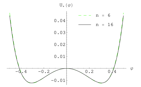
Figure 1: Approximate fixed point effective potential $U_{\ast}(\varphi)$ and the corresponding deviation of the right hand side of eq. (10) from constant, for $n=6$ and $n=16$ ($\varphi_{\rm max}=0.5$ in both cases; the two graphs for $U_{\ast}(\varphi)$ are hardly distinguishable).

At this stage the odd coefficients of expansion (11) are zero, and minimization involves $n/2$ even coefficients of (11), plus $F_{0}$. The achievable proximity of $F(\varphi)$ to constant is improving rapidly with the increasing order of the approximation (Fig. 1).

The next step is the study of deviations of $U(\varphi)$ from $U_{\ast}(\varphi)$, and their evolution over $t$. As will be clear below, it is convenient to introduce a separate set of parameters, $b_{i}=b_{i}^{\ast}+\delta b_{i}$, $i=1\ldots n$, to parameterize the deviation of $U$ from $U_{\ast}$ (which corresponds to $b_{i}^{\ast}$). Then the evolution of parameters follows from

$${\partial\over\partial t}U(b_{i}^{\ast}+\delta b_{i})=F(b_{i}^{\ast}+\delta b_{i})-F_{\ast}.$$ (13)

We have to subtract $F_{\ast}\equiv F(b_{i}^{\ast})$ in the right hand side, to account for the approximate nature of our treatment of the fixed point. Thus

$${\partial U\over\partial b_{j}}{d\over dt}\delta b_{j}={\partial F\over\partial b_{j}}\delta b_{j}.$$ (14)

Here $\partial U/\partial b_{j}$ and $\partial F/\partial b_{j}$ are understood to be taken at the fixed point, $b_{i}^{*}$. Defining the scalar product

$$\langle f_{1}(\varphi)|f_{2}(\varphi)\rangle={1\over 2\varphi_{\rm max}}\int_{-\varphi_{\rm max}}^{\varphi_{\rm max}}f_{1}(\varphi)f_{2}(\varphi)d\varphi,$$ (15)

and introducing matrices

$$A_{ij}=\biggl{\langle}{\partial U\over\partial b_{i}}\biggl{|}{\partial U\over\partial b_{j}}\biggr{\rangle},\quad B_{ij}=\biggl{\langle}{\partial U\over\partial b_{i}}\biggl{|}{\partial F\over\partial b_{j}}\biggr{\rangle},$$ (16)

we obtain

$$A\cdot{d\over dt}\vec{\delta b}=B\cdot\vec{\delta b}.$$ (17)

Thus

$$\vec{\delta b}=\sum_{i=1}^{n}c_{i}e^{\lambda_{i}t}\vec{v}_{i},$$ (18)

where $\lambda_{i}$ and $\vec{v}_{i}$ are, respectively, eigenvalues and eigenvectors of $A^{-1}B$. $\lambda_{i}$ are exactly the critical exponents we are interested in.

To simplify the computation and improve its numerical stability, we parameterize the deviation of $U$ from $U_{\ast}$ so that $A_{ij}=\delta_{ij}$, namely,

$$U(\varphi)=U_{\ast}(\varphi)+\sum_{j=1}^{n}b_{j}\tilde{P}_{j}(\varphi),$$ (19)

where $\tilde{P}_{j}(\varphi)$ are Legendre polynomials $P_{j}$ normalized on $[-\varphi_{\rm max},\varphi_{\rm max}]$:

$$\tilde{P}_{j}(\varphi)=\sqrt{2j+1\over 2\varphi_{\rm max}}P_{j}\left({\varphi\over\varphi_{\rm max}}\right).$$ (20)

Then $\lambda_{i}$ are just the eigenvalues of the matrix $B$.

4 Results

The results for critical exponents are collected in Tables 1–3. We use polynomial approximations of order $6\ldots 16$, for three values of $\varphi_{\rm max}$: 0.5, 0.44 and 0.4. We observe that the higher eigenvalues are almost insensitive to the choice of $\varphi_{\rm max}$. This is fortunate, and provides additional evidence that the LPA captures correctly the important part of physics. The usual approach relies on avoiding the singularity at large $\varphi$ [14, 19, 20, 15], and one may wonder to what extent the results are determined by the asymptotical properties of the WH equation at large $\varphi$, rather than by properties at physically relevant range of $\varphi$ (of order of the position of the minimum of $U_{\ast}$).

Our values of the critical exponents in the even sector,

$$y_{t}\approx 1.45041,\ \omega\approx 0.5952,\ \omega_{2}\approx 2.838,\ \omega_{3}\approx 5.18,$$ (21)

are in agreement with the most accurate of the previous computations [19]:

$$\nu\approx 0.6895,\ \omega\approx 0.5952,\lambda_{2}\approx-2.8384,\lambda_{3}\approx-5.1842.$$ (22)

The most interesting part of our results is the set of critical exponents for the odd sector:

$$y_{h}=2.5,\ y_{\rm shift}=0.5,\ \omega_{A}\approx 1.691,\ \omega_{A2}\approx 4.00.$$ (23)

The appearance of the somewhat unusual exponent $y_{\rm shift}$ reflects the fact that, strictly speaking, in the case of asymmetric $U(\varphi)$ the renormalization group transformation should include, in addition to blocking and rescaling of $\varphi$, also the shift of $\varphi$. As we did not take this into account, this additional exponent emerged.

The value of $\omega_{A}$ is consistent with [21] but has higher precision. We are not aware of any previous computation of $\omega_{A2}$.

To summarize, we have computed the critical exponents, in $\varphi$-even as well as in $\varphi$-odd sectors, for the systems in the 3D Ising universality class, in the local potential approximation. We show that the previously known values of the critical exponents in the $\varphi$-even sector are reproduced, within our accuracy, even without relying upon avoiding the singularity in the Wegner-Houghton equation at $\varphi\to+\infty$. The absence of slowly-decaying $\varphi$-odd corrections to scaling implies that they are not responsible for asymmetries observed in Monte Carlo studies [7].

I am deeply grateful to Prof. H. Neuberger for his kind hospitality, support, and many interesting discussions. I would like to thank the Department of Physics and Astronomy, Rutgers University and the School of Natural Sciences, IAS, for their hospitality and support. This work was supported in part by DOE grants DE-FG02-96ER40949 and DE-FG02-90ER40542.

$n$		16	14	12	10	8	6
$\sigma$		${\scriptstyle 1.48\times 10^{-8}}$	${\scriptstyle 2.36\times 10^{-7}}$	${\scriptstyle 8.48\times 10^{-7}}$	${\scriptstyle 2.31\times 10^{-6}}$	${\scriptstyle 4.13\times 10^{-5}}$	${\scriptstyle 2.78\times 10^{-4}}$
$y_{h}$	$A$	2.5	2.5	2.5	2.5	2.5	2.5
$y_{t}$	$S$	1.450413	1.450412	1.450402	1.45044	1.44878	1.44099
$y_{\rm shift}$	$A$	0.5	0.500003	0.500035	0.500223	0.505546	0.491122
$-\omega$	$S$	-0.595235	-0.595256	-0.595119	-0.595044	-0.589349	-0.530546
$-\omega_{A}$	$A$	-1.69132	-1.6914	-1.69099	-1.70327	-1.5294	-0.920653
$-\omega_{2}$	$S$	-2.83838	-2.83869	-2.83794	-2.89125	-2.50668	-2.00335
$-\omega_{A2}$	$A$	-3.99828	-4.00259	-4.11481	-3.46038	-3.38734
$-\omega_{3}$	$S$	-5.18418	-5.20558	-5.37167	-4.48014	-5.0081
	$A$	-6.44866	-6.64226	-5.61029	-6.89618
	$S$	-7.76251	-7.95578	-6.91652	-9.08612
	$A$	-9.35137	-8.46459	-11.5582
	$S$	-10.8738	-10.2681	-14.3183
	$A$	-12.3235	-17.3682
	$S$	-14.6305	-20.7111
	$A$	-24.3498
	$S$	-28.2887

Table 1: Critical exponents for $\varphi_{\rm max}=0.5$. The quality of approximation is characterized by $\sigma$, according to (12). Second column indicates the symmetry of the eigenvector ($S$ = even, $A$ = odd).

$n$		16	14	12	10	8	6
$\sigma$		${\scriptstyle 3.41\times 10^{-9}}$	${\scriptstyle 3.96\times 10^{-8}}$	${\scriptstyle 3.14\times 10^{-7}}$	${\scriptstyle 3.43\times 10^{-7}}$	${\scriptstyle 1.41\times 10^{-5}}$	${\scriptstyle 1.28\times 10^{-4}}$
$y_{h}$	$A$	2.5	2.5	2.5	2.5	2.5	2.5
$y_{t}$	$S$	1.450410	1.45035	1.45056	1.4505	1.44882	1.45284
$y_{\rm shift}$	$A$	0.499991	0.499918	0.500252	0.500054	0.498699	0.523208
$-\omega$	$S$	-0.595165	-0.595677	-0.594694	-0.593543	-0.604152	-0.546673
$-\omega_{A}$	$A$	-1.69158	-1.69361	-1.68492	-1.7014	-1.75849	-1.92471
$-\omega_{2}$	$S$	-2.83969	-2.84017	-2.83152	-2.90894	-3.08336	-3.59606
$-\omega_{A2}$	$A$	-3.99407	-4.03145	-4.2279	-4.56781	-5.65287
$-\omega_{3}$	$S$	-5.19053	-5.32954	-5.73614	-6.33275	-8.01733
	$A$	-6.77786	-7.47611	-8.36842	-10.7213
	$S$	-8.44641	-9.46912	-10.6988	-13.8132
	$A$	-11.7329	-13.3336	-17.2785
	$S$	-14.2826	-16.2727	-21.1253
	$A$	-19.5243	-25.361
	$S$	-23.0967	-29.9828
	$A$	-34.9966
	$S$	-40.4086

Table 2: Critical exponents for $\varphi_{\rm max}=0.44$.

$n$		16	14	12	10	8	6
$\sigma$		${\scriptstyle 1.65\times 10^{-9}}$	${\scriptstyle 6.53\times 10^{-9}}$	${\scriptstyle 1.15\times 10^{-7}}$	${\scriptstyle 3.14\times 10^{-7}}$	${\scriptstyle 5.78\times 10^{-6}}$	${\scriptstyle 6.64\times 10^{-5}}$
$y_{h}$	$A$	2.5	2.5	2.5	2.5	2.5	2.5
$y_{t}$	$S$	1.45031	1.45014	1.45136	1.45019	1.44437	1.47603
$y_{\rm shift}$	$A$	0.499857	0.499766	0.501045	0.499452	0.493915	0.537914
$-\omega$	$S$	-0.595091	-0.597076	-0.593018	-0.590154	-0.619136	-0.6057
$-\omega_{A}$	$A$	-1.69522	-1.6978	-1.66645	-1.73619	-2.07471	-2.76637
$-\omega_{2}$	$S$	-2.84795	-2.83693	-2.82088	-3.05967	-3.72532	-4.91745
$-\omega_{A2}$	$A$	-3.98292	-4.09967	-4.59586	-5.64517	-7.68927
$-\omega_{3}$	$S$	-5.20884	-5.56624	-6.46	-7.98584	-10.7612
	$A$	-7.30803	-8.68827	-10.7014	-14.2306
	$S$	-9.3943	-11.2751	-13.8281	-18.2123
	$A$	-14.2416	-17.3769	-22.65
	$S$	-17.6035	-21.3259	-27.5739
	$A$	-25.6903	-32.9993
	$S$	-30.4805	-38.8901
	$A$	-45.2637
	$S$	-52.1331

Table 3: Critical exponents for $\varphi_{\rm max}=0.4$.

References

- [1] A. Pelissetto and E. Vicari, Critical Phenomena and Renormalization-Group Theory, cond-mat/0012164.
- [2] J.F. Nicoll and R.K.P. Zia, Phys. Rev. B 23 (1981) 6157; J.F. Nicoll, Phys. Rev. A 24 (1981) 2203.
- [3] J.J. Rehr and N.D. Mermin, Phys. Rev. A 8 (1973) 472.
- [4] A.D. Bruce and N.B. Wilding, Phys. Rev. Lett. 68 (1992) 193; N.B. Wilding and A.D. Bruce, J. Phys.: Cond. Mat. 4 (1992) 3087; N.B. Wilding, Phys. Rev. E 52 (1995) 602 [cond-mat/9503145]; N.B. Wilding and M. Müller, J. Chem. Phys. 102 (1995) 2562 [cond-mat/9410077]; N.B. Wilding, J. Phys.: Cond. Mat. 9 (1997) 585 [cond-mat/9610133].
- [5] D.A. Kirzhnits and A.D. Linde, Phys. Lett. B 42 (1972) 471; Ann. Phys. 101 (1976) 195.
- [6] K. Kajantie, M. Laine, K. Rummukainen and M. Shaposhnikov, Phys. Rev. Lett. 77 (1996) 2887 [hep-ph/9605288].
- [7] K. Rummukainen, M. Tsypin, K. Kajantie, M. Laine and M. Shaposhnikov, Nucl. Phys. B532 (1998) 283 [hep-lat/9805013].
- [8] M.A. Halasz, A.D. Jackson, R.E. Shrock, M.A. Stephanov and J.J.M. Verbaarschot, Phys. Rev. D 58 (1998) 096007 [hep-ph/9804290]; J. Berges and K. Rajagopal, Nucl. Phys. B 538 (1999) 215 [hep-ph/9804233]; M. Stephanov, K. Rajagopal and E. Shuryak, Phys. Rev. Lett. 81 (1998) 4816 [hep-ph/9806219].
- [9] Z. Fodor and S.D. Katz, hep-lat/0106002; hep-lat/0110102.
- [10] F.J. Wegner, Phys. Rev. B 6 (1972) 1891.
- [11] F.C. Zhang and R.K.P. Zia, J. Phys. A 15 (1982) 3303.
- [12] K.E. Newman and E.K. Riedel, Phys. Rev. B 30 (1984) 6615.
- [13] F.J. Wegner and A. Houghton, Phys. Rev. A 8 (1973) 401.
- [14] A. Hasenfratz and P. Hasenfratz, Nucl. Phys. B 270 [FS16] (1986) 687.
- [15] C. Bagnuls and C. Bervillier, Phys. Reports 348 (2001) 91 [hep-th/0002034].
- [16] J. Berges, N. Tetradis and Ch. Wetterich, Phys. Reports, to appear [hep-ph/0005122].
- [17] A. Parola and L. Reatto, Phys. Rev. Lett. 53 (1984) 2417; Phys. Rev. A 31 (1985) 3309.
- [18] C. Bagnuls and C. Bervillier, Phys. Rev. B 41 (1990) 402.
- [19] J. Comellas and A. Travesset, Nucl. Phys. B 498 (1997) 539.
- [20] C. Bagnuls and C. Bervillier, Cond. Matt. Phys. 3 (2000) 559.
- [21] C. Bagnuls, C. Bervillier and M. Shpot, unpublished, as quoted in [15].