Investigating QCD Vacuum on the lattice

Abstract

Investigations on the structure of QCD vacuum from first principles can be done on the lattice. The mechanism of confinement is an example: results from lattice on it are reviewed.

1 Introduction

Euclidean Feynman path integral uniquely identifies the ground state of a field theory (vaccum)[1].

The Feynman functional integral is defined as the limit of ordinary integrals defined on discrete set of points in a four dimensional box, when the number of points is sent to infinity filling the box densely; the size of the box is then sent to infinity to cover the whole space time. Lattice formulation is an approssimant in this sequence.

QCD has an UV fixed point at $g=0$ (asymptotic freedom): as $g\to 0$ the physical length scale $\xi$ increases in units of the lattice spacing $a$

$$\frac{a}{\xi}\mathop{\rightarrow}_{g_{0}\to 0}=0$$ (1)

The density of lattice points in physical units goes large. On the other hand a mass gap exists in the theory, which makes the infinite volume limit well defined as a thermodynamical limit.

Lattice is a good approximant of QCD if

$$a\ll\xi\ll La$$ (2)

with $L$ the size of the lattice.

The above argument is a strong indication that QCD most probably exists as a field theory in the constructive sense, and can be defined as a limit of lattice formulation as $g_{0}\to 0$, and $L$ is such that the inequality (2) is satisfied.

The textbook quantization of QCD is based on perturbation theory, and the ground state is Fock vacuum of quarks and gluons.

Phenomenological evidence exists[2] that the QCD vacuum is not the perturbative vacuum. The instability of Fock’s vacuum is possibly the origin of the non Borel summability of the perturbative expansion[3].

Perturbation theory apparently works at small distances but is not well defined and is unable to describe large distance physics.

The most clear evidence that Fock vacuum is not a good approximation to QCD ground state, is that its elementary excitations, quarks and gluons, have never been observed as free particles. This phenomenon is known as confinement of colour and is one of the most intriguing properties of QCD.

The study of the mechanism of confinement is an important chapter of the investigation of the structure of QCD vacuum on the lattice, and will be the object of this talk. In sect.2 I will review the experimental evidence for confinement. In sect.3 I will discuss the phenomenology of the deconfinement transition as observed in numerical simulations on the lattice. This will naturally lead us to the idea of duality, which will be the object of sect.4. Progress in understanding confinement as dual superconductivity of the vacuum will be reviewed in sect.5

2 Confinement: experimental evidence.

Confinement is defined as the absence of colored particles in asymptotic states.

The existing experimental evidence for confinement is based on the negative result of searches of fractionally charged particles (quarks) in particle reactions and in nature.

The cross section $\sigma_{q}$ for the inclusive production of quark or antiquark in the process

$$p+p\to q(\bar{q})+X$$

at c.m. energies $\sim 100$ GeV has an upper limit[4]

$$\sigma_{q}<10^{-40}\,\rm{cm}^{2}$$

to be compared with the total cross section $\sigma_{T}$ at the same energy $\sigma_{T}\sim 10^{-25}\,{\rm cm}^{2}$.

The ratio $R_{q}=\sigma_{q}/\sigma_{T}$ has then the upper bound

$$R<10^{-15}$$

while the expected value in the absence of confinement is a sizable fraction of unity.

The negative result of the search of fractionally charged particles in ordinary matter by Millikan-like experiments gives an upper limit for the ratio $R$ of the quarks abundance $n_{q}$ to nucleons abundance $n_{p}$

$$R_{ob}=\frac{n_{q}}{n_{p}}<10^{-27}$$

corresponding to the analysis of $\sim 1$ gr of matter.

In the absence of confinement the expectation for $R$, $R_{SCM}$, in the standard cosmological model is $R_{SCM}\sim 10^{-12}$[5]. Again

$$R/R_{SCM}<10^{-15}$$

A ratio smaller than $10^{-15}$, if different from zero, would be too small to have a natural explanation in any theory. The most natural interpretation is then that those ratios are strictly zero, or that confinement is an absolute property of the vacuum based on a symmetry[6].

The question is: what symmetry of QCD vacuum prevents quarks to exist as free particles?

As for gluons, they have no such characteristic signature as a fractional charge, and their identification is not clearly feasible. No experimental data exist on gluon confinement. We shall define anyhow confinement as absence of any colored particle as a free particle.

3 Deconfinement Phase transition on the lattice.

QCD at finite temperature can be studied on the lattice. The partition function $Z(T)$ of a field with action $S[\Phi]$ is equal to the Feynman integral in Euclidean space, with the time direction extending from 0 to $1/T$ and periodic boundary conditions in time for bosons, antiperiodic for fermions

$$Z(T)=\int\Pi[{\cal D}\Phi]e^{-\beta\!\int\!d^{3}x\int_{0}^{1/T}\hskip-5.0ptdx_{0}S_{E}[\Phi(\vec{x},x_{0})]}$$ (3)

In lattice QCD this corresponds to having a lattice of size $N_{S}^{3}\times N_{T}$, with $N_{S}\gg N_{T}$, and the temperature is given by the inverse of the temporal extension $N_{T}a$ ($a$ the lattice spacing).

The value of $a$ in physical units depends on the coupling constant ($\beta=2N/g^{2}$) via renormalization group

$$a(\beta)=\frac{1}{\Lambda_{L}}\exp(-b_{0}\beta)$$

with

$$b_{0}>0\qquad\hbox{(asymptotic freedom)}$$

Hence

$$T=\frac{1}{N_{T}a}=\frac{\Lambda_{L}}{N_{T}}\exp(b_{0}\beta)$$ (4)

As a consequence of asymptotic freedom low temperature (confinement) corresponds to strong coupling (large $g$) or to disorder in the language of statistical mechanics, high temperature corresponds to order or to weak couling.

If confinement is due to a symmetry, it has to be a symmetry of the disordered phase. This naturally leads to the idea of duality, which will be the object of sect.3.

The deconfinement transition is detected on the lattice in pure gauge theory, by looking at the correlator

$${\cal D}(\vec{x}-\vec{y})=\langle L(\vec{x})L(\vec{y})\rangle$$ (5)

where $L(\vec{x})$, the Polyakov line, is the trace of the parallel transport along the time axis across the lattice and back via periodic boundary conditions

$$L(\vec{x})=Tr\left\{P\exp\left(i\int_{0}^{aN_{T}}\hskip-3.0ptA_{0}(\vec{x},x_{0})dx^{0}\right)\right\}$$ (6)

The static potential between a $q\,\bar{q}$ pair is given by

$$V_{q\bar{q}}(\vec{x}-\vec{y})=\frac{\ln{\cal D}(\vec{x}-\vec{y})}{aN_{T}}$$ (7)

By cluster property, at large distances

$${\cal D}(\vec{x}-\vec{y})\simeq C\exp(-A|\vec{x}-\vec{y}|aN_{T})+K|\langle L\rangle|^{2}$$ (8)

A critical temperature $T_{c}$ is observed such that

$$\begin{array}[]{lccl}\rm{for}\,T<T_{c}&\langle L\rangle=0&V(r)\mathop{=}\limits_{r\to\infty}\sigma r&\rm{(conf.)}\\ \rm{for}\,T>T_{c}&\langle L\rangle\neq 0&V(r)\mathop{=}\limits_{r\to\infty}0&\rm{(deconf.)}\end{array}$$

Confinement is related to the presence of a linear potential at large distances: $\sigma$ is known as string tension.

For $SU(2)$ gauge theory the phase transition at $T_{c}$ is second order,and belongs to the universality class of the $3d$ Ising model. $T_{c}\simeq 180\,{\rm{MeV}}$[7].

For $SU(3)$ gauge theory the transition is weak first order, and $T_{c}\simeq 270\,{\rm{MeV}}$[8].

In the presence of quarks the symmetry $Z_{N}$ of which $L$ is an order parameter, is not a symmetry any more. For massless quarks a chiral symmetry exists above some temperature $T_{c}$, which is spontaneously broken for $T<T_{c}$, the pseudoscalar octet being the Goldstone particles. For $m_{q}\neq 0$ the chiral symmetry is again explicitely broken.

It is qualitatively clear that confinement can produce a breaking of chiral symmetry: in a bag model chirality is inverted in the reflection on the confining wall. Numerical indications also exist that the two transitions take place at the same temperature. However the overall situation is not satisfactory.

First of all if a phase exist in which color is confined, and a phase at higher temperature in which quarks and gluons are free particles, an exact order parameter should exist for this transition.

In addition a strong theoretical hint exists that, when the number of colors $N_{c}$ is sent large, with the constraint $N_{c}g^{2}=\lambda$ fixed, a limiting theory is defined, which does not differ much in its physical content from the realistic theory where $N_{c}=3$.

The expansion in $1/N_{c}$ should be a convergent expansion[9].

In this philosophy quark loops are non leading ${\cal O}(1/N_{c})$ and therefore the physics of confinement, i.e. the symmetry, should be the same as in quenched approximation.

4 Duality[10].

Duality is a deep concept in field theory, in statistical mechanics, in string theory. It applies to systems in $d+1$ dimensions having non local topological excitations in $d$ dimensions. Two complementary descriptions can be given of such systems.

A direct description, in terms of local fields $\Phi$, in which topological excitations $\mu$ are non local. Symmetry is described by order parameters, the v.e.v. $\langle\Phi\rangle$ of the fields $\Phi$. This description is convenient in the ordered phase, or weak coupling regime.

A dual description in which $\mu$ are local operators, and $\Phi$ non local excitations. Symmetry is described by disorder parameters $\langle\mu\rangle$. The dual coupling is $g_{D}\sim 1/g$. This description maps the strong coupling regime of the direct theory into the weak coupling regime of the dual. Therefore it is convenient in the strong coupling regime.

The prototype system[11] with duality is the $1+1$ dimensional Ising model: there the field $\Phi$ is the spin variable $\sigma(i)=\pm 1$. The dual configurations $\mu$ are 1 dimensional kinks. The dual description is again an Ising model in which the creation operator of a kink is $\mu(i)=\pm 1$ and the dual Boltzman factor $\beta_{D}$ is defined by the relation

$$\sinh 2\beta=\frac{1}{\sinh 2\beta_{D}}$$ (9)

or $\beta\sim 1/\beta_{D}$. In the model $T=1/\beta$ plays the role of the coupling constant.

Other examples are

• The 3d $XY$ model[12], which belongs to the class of universality of liquid $He_{4}$. The topological excitations are abelian vortices.

• The Heisenberg magnet, where the topological excitations are $2d$ Weiss-domains[13].

• the $N=2$ SUSY QCD[14] where the excitations are monopoles.

• Superstring $M$ theories[15].

• Compact $U(1)$ gauge theories, where the topological excitations are monopoles[16, 17].

The question is: what are the dual excitations in QCD?

Two proposals exist in the literature, both due to G. t’Hooft[6, 18].

• Monopoles. Monopole condensation in the vacuum produces dual superconductivity, and confinement of electric charges via Abrikosov flux lines (Meissner effect). Monopoles are defined by a procedure named “abelian projection”[18] based on the choice of a local operator in the adjoint representation, as discussed below. In a sense the mechanism is largely undefined, since there is a continuous infinity of choices for the operator used to define the monopoles and their interrelation is not understood. A guess is that all these choices are physically equivalent[18].

  The positive feature is that confinement is explained in a simple form: the chromoelectric field of a $q\bar{q}$ pair is channeled into an Abrikosov flux tube with energy proportional to the length, i.e. to the distance $r$ between the pair[19, 20]

  $$V(R)=\sigma R$$

  $\sigma$, the energy per unit length of the tube, is the string tension.

• Vortices. A vortex is a magnetic defect associated to a closed line $C$. The operator $B(C)$ which creates a vortex at some time $t$, obeys the following algebra, with the operator $W(C^{\prime})$ creating a Wilson loop along the line $C^{\prime}$

  $$B(C)W(C^{\prime})=W(C^{\prime})B(C)\exp\left(i\frac{n_{CC^{\prime}}}{N}2\pi\right)$$

  where $n_{CC^{\prime}}$ is the winding number of the lines $C,C^{\prime}$. It can be shown that, whenever $\langle W(C^{\prime})\rangle$ obeys the area law, $\langle W(C^{\prime})\rangle\sim\exp(-Area_{C^{\prime}})$, as the loop goes large, $\langle B(C)\rangle$ obeys the perimeter law, and viceversa if $\langle B(C)\rangle$ obeys the area law, $\langle W(C^{\prime})\rangle$ obeys the perimeter law.

  Area law implies that $\langle L\rangle$, the expectation value of the Polyakov line vanishes. One can define a dual Polyakov line $L^{\prime}$ wich is a vortex along a straight path crossing space from $-\infty$ to $+\infty$. Then for $T<T_{c}$, $\langle L\rangle=0$, for $T>T_{c}$, $\langle L^{\prime}\rangle=0$. $\langle L^{\prime}\rangle$ is a disorder parameter for confinement[21].

The definition of monopoles is associated to the choice of an operator $\vec{\Phi}(x)$ in the adjoint representation: we will speak of $SU(2)$ gauge group for simplicity, but the procedure is easily generalized to $SU(N)$. Let $\hat{\Phi}(x)\equiv\vec{\Phi}(x)/|\vec{\Phi}(x)|$ be the direction of $\vec{\Phi}$ in color space. A gauge invariant field strength $F_{\mu\nu}$ can be defined as[22]

$$F_{\mu\nu}=\hat{\Phi}\cdot\vec{G}_{\mu\nu}-\frac{1}{g}\hat{\Phi}(D_{\mu}\hat{\Phi}\wedge D_{\nu}\hat{\Phi})$$ (10)

$$\vec{G}_{\mu\nu}=\partial_{\mu}\vec{A}_{\nu}-\partial_{\nu}\vec{A}_{\mu}+g\vec{A}_{\mu}\wedge\vec{A}_{\nu}$$

$$D_{\mu}=\partial_{\mu}-g\vec{A}_{\mu}\wedge$$

The two terms in the definition (10) are separately gauge invariant and color singlets: they are arranged in such a way that bilinear terms $A_{\mu}A_{\nu}$ or $A_{\mu}\partial_{\nu}\Phi$ cancel. Indeed

$$F_{\mu\nu}=\hat{\Phi}(\partial_{\mu}\vec{A}_{\nu}-\partial_{\nu}\vec{A}_{\mu})-\frac{1}{g}\hat{\Phi}(\partial_{\mu}\hat{\Phi}\wedge\partial_{\nu}\hat{\Phi})$$ (11)

The gauge transformation bringing $\Phi$ in the same direction (say (0,0,1)) in color space is called abelian projection. After abelian projection

$$F_{\mu\nu}=\partial_{\mu}A^{3}_{\nu}-\partial_{\nu}A^{3}_{\mu}$$ (12)

The source of the dual tensor $F^{*}_{\mu\nu}=1/2\varepsilon_{\mu\nu\rho\sigma}F^{\rho\sigma}$ is a magnetic current

$$j_{\nu}=\partial^{\mu}F^{*}_{\mu\nu}$$ (13)

and is conserved. The corresponding $U(1)$ magnetic symmetry can either be Wigner, and then a magnetic charge operator is defined and Hilbert space is superselected, or be Higgs broken, which implies the existence of at least one magnetically charged operator $\mu$ such that $\langle\mu\rangle\neq 0$. $\langle\mu\rangle\neq 0$ implies dual superconductivity. Notice that in a noncompact formulation $j^{\nu}=0$ (Bianchi identities).

In principle the existence of dual superconductivity can be investigated in any abelian projection by looking at the v.e.v. $\langle\mu\rangle$ of an operator creating a magnetic charge in that abelian projection.

5 Construction of the disorder parameter $\langle\mu\rangle$[23, 24, 25, 26]

Once the dual topological excitations are identified the disorder parameter can be constructed as the v.e.v. of their creation operator $\mu$. The construction of $\mu[\Phi]$ interms of the field of the direct description $\Phi$ is an explicit realization of the duality transformation.

The guiding idea goes back to ref.[27] and amounts to a traslation of the fields in the Schrödinger picture by the classical topological configuration. In the same way as

$$e^{ipa}|x\rangle=|x+a\rangle$$ (14)

$$\mu(x)=\exp\left(i\int d^{3}y\Pi(x_{0},\vec{y})\bar{\varphi}(\vec{y}-\vec{x})\right),$$ (15)

with $\Pi$ the conjugate momentum to the field $\Phi$

$$\left[\Phi(x_{0},\vec{x}),\Pi(x_{0},\vec{y})\right]=i\delta^{3}(\vec{x}-\vec{y}),$$

adds $\bar{\varphi}(\vec{x})$ to the field configuration

$$\mu(\vec{x})|\Phi(\vec{x})\rangle=|\Phi(\vec{x})+\bar{\varphi}(\vec{x})\rangle$$

Adapting the above construction to a compact formulation of the theory as in QCD on the lattice is far from trivial, but has been done[24, 25, 26].

A correct,gauge invariant, definition of the operator $\mu$ for abelian projected monopoles exists[24]. The resulting operator is a Dirac like magnetically charged and gauge invariant operator, which can then have non vanishing v.e.v. without violating gauge invariance[28].

The construction has been checked on systems already studied and understood by other methods, starting with the 2d Ising model[29], where our operator $\mu$ which creates kinks does indeed coincide with the dual variable $\sigma^{*}$ of ref.[11].

For the 3d $XY$ model the phase transition was always conjectured to be produced by condensation of vortices, but that condensation was detected in numerical simulations by observing an increase of the number of vortices in condensed phase: our construction shows that $\langle\mu\rangle\neq 0$, or that the number of vortices is not defined in the vacuum of the condensed phase[12].

For the Heisenberg model we have found[13] that the Curie transition can be looked as an order disorder transition, and that the high temperature phase is ordered in the dual language, by condensation of non abelian $O(3)$ vortices.

A numerical problem has also been solved; $\mu$ defined by eq.(15) is the exponential of an integral over the spatial volume: therefore it fluctuates typically as $\exp(L^{3/2})$, which is a wild fluctuation. In fact the disorder parameter $\langle\mu\rangle$ is the ratio of two partition functions

$$\langle\mu\rangle=\frac{\tilde{Z}}{Z}$$

and has the fluctuations typical of a partition function. $Z$ is the ordinary partition function of the theory, and $\tilde{Z}=\int e^{-\tilde{S}}$ corrisponds to a modification of the action coming from the exponent in $\mu$, eq.(15).

A way out of this difficulty consists[30, 23] in considering instead of $\langle\mu\rangle$ the quantity

$$\rho=\frac{d}{d\beta}\ln\langle\mu\rangle=\langle S\rangle_{S}-\langle{\tilde{S}}\rangle_{\tilde{S}}$$ (16)

$\beta=\frac{2N}{g^{2}}$, which contains all the relevant information of $\langle\mu\rangle$.

A typical shape of $\langle\mu\rangle$ is shown in fig.1. The corresponding $\rho$ is shown in fig.2. The peak seats on the location of the phase transition.

Figure 1: $\langle\mu\rangle$ for compact $U(1)$.

Figure 2: $\rho$ for compact $U(1)$

The phase transition in principle takes place at infinite volume. The limit can be performed by a finite size scaling analysis as follows; if $\delta$ is the critical index of $\mu$ and $\tau=(1-T/T_{c})$ the reduced temperature,

$$\langle\mu\rangle\mathop{\simeq}_{\tau\to 0}\tau^{\delta}$$

then

$$\langle\mu\rangle\mathop{\simeq}_{\tau\to 0}\tau^{\delta}\Phi(\frac{a}{\xi},\frac{L}{\xi})$$ (17)

The functional dipendence is dictated by the fact that $\Phi$ is dimensionless: $a$ is the lattice spacing, $\xi$ the correlation length, $L$ the extension of the lattice. As $\tau\to 0$, $\xi$ goes large with a critical index $\nu$

$$\xi\propto\tau^{-\nu}$$

$a/\xi$ can be approximated with 0 (scaling limit), and $L/\xi$ can be traded with $L^{1/\nu}\tau$. Hence

$$\langle\mu\rangle\sim\tau^{\delta}f(L^{1/\nu}\tau)$$

and

$$\rho L^{-1/\nu}=\frac{\delta}{\tau L^{1/\nu}}+f^{\prime}(L^{1/\nu}\tau)$$ (18)

$\rho/L^{1/\nu}$ is a universal function of $L^{1/\nu}\tau$, i.e. it scales when plotted versus $L^{1/\nu}\tau$.

Since this scaling law is valid for the appropriate value of $\nu$ and $\beta_{c}$, the determination of $\nu$, $\beta_{c}$ and $\delta$ is then possible.

6 Results for QCD[24, 25, 26].

$\langle\mu\rangle$, or better $\rho$, has been studied for pure gauge $SU(2)$ and $SU(3)$ gauge theories across the deconfining phase transition, in a number of different abelian projections.

A clear evidence has been obtained that, irrespective of the choice of the abelian projection

• $\langle\mu\rangle\neq 0$ in the confined phase ($T<T_{c}$).

• $\langle\mu\rangle\sim\exp(-kL_{S})$, $k>0$ for $T>T_{c}$, $L_{S}$ being the spatial extension of the lattice. This means $\langle\mu\rangle=0$ at $T>T_{c}$ in the thermodynamical limit.

• $$\langle\mu\rangle\mathop{\sim}_{T\to T_{c}^{-}}\left(1-\frac{T}{T_{c}}\right)^{\delta}$$

• $T_{c}$ and $\nu$ can be determined, together with $\delta$ from the finite size scaling analysis sketched in sect.3.

Fig.3 shows a typical form of $\rho$ as a function of $\beta$ for different lattice sizes and $SU(2)$ gauge theory.

Fig.4 shows the quality of the scaling equation (18), i.e. the validity of the extrapolation at infinite volume.

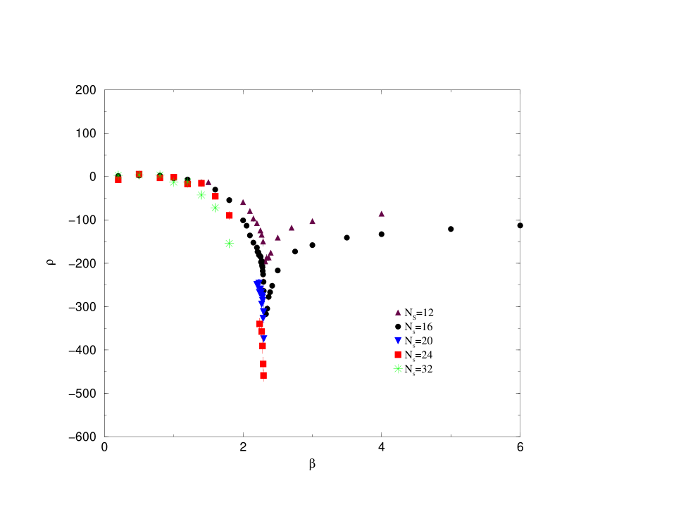
Figure 3: $\rho$ for monopole condensation in $SU(3)$.

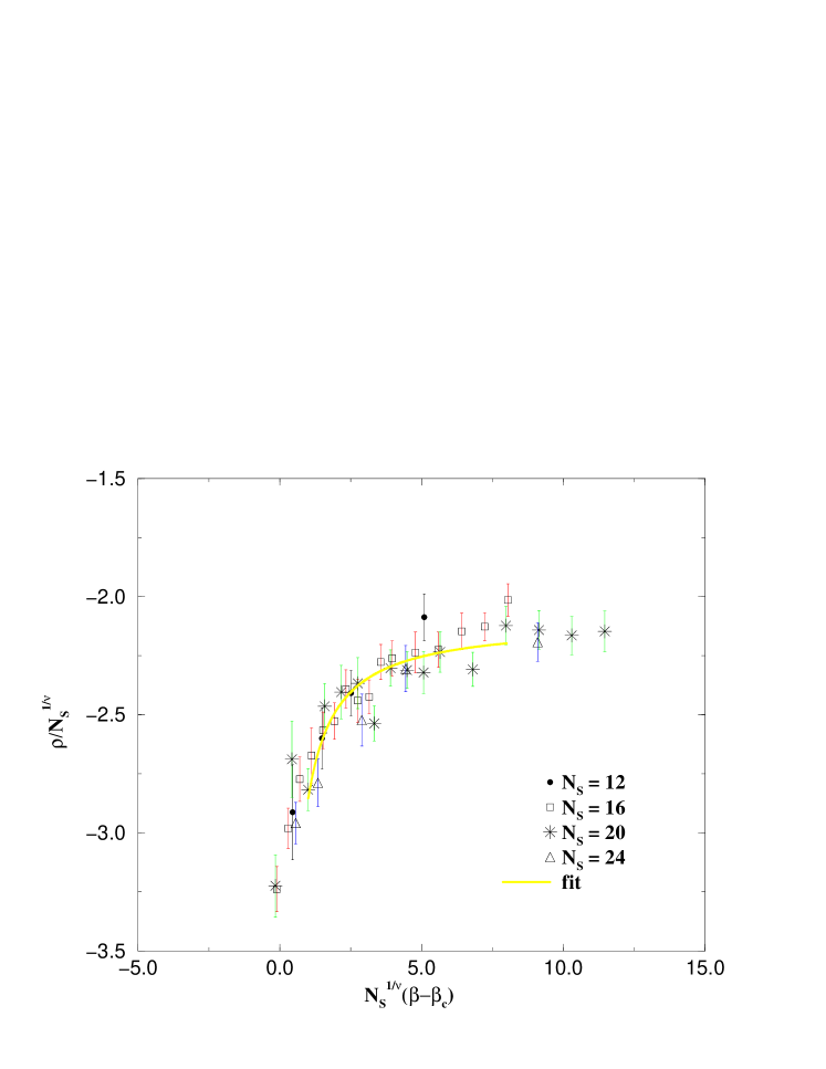
Figure 4: Finite size scaling of $\rho$.

$T_{c}$ agrees with the determination made using the traditional order parameter $\langle L\rangle$, and so does $\nu$. For $SU(2)$ $\nu=0.62(2)$ in agreement with the expectation that the transition belongs to the universality class of the 3d Ising model, $\delta=.20(8)$.

For $SU(3)$, $\nu=1/3$, which means that the transition is first order, even if weak enough to allow a scaling region, and $\delta=.50(3)$.

The independence of the result from the choice of the abelian projection has been checked by performing the analysis in a number of different abelian projections, but also averaging on a very large number (infinite) of abelian projections[26].

These results clearly indicate that confining vacuum is a dual superconductor.

The same disorder parameter $\langle\mu\rangle$ can be used in full $QCD$ (including dynamical quarks) where it is well defined, contrary to $\langle L\rangle$ whose symmetry $Z_{N}$ is explicitely broken by the very presence of quarks and to $\langle\bar{\psi}\psi\rangle$, whose symmetry is broken by quark masses.

The analysis for full QCD is in progress and of course requires a big computational effort. There the dependence on the masses of the quarks makes the finite size scaling analysis, eq.(18) more complicated. Preliminary results[31], however, indicate that also in full QCD there is a transition from dual superconductor to normal across the transition. If these preliminary indications get confirmed by the quantitative analysis which is on the way, we would have a good order parameter for confinement, even in the presence of (massive) quarks. In principle the two transitions, chiral and deconfinement, could take place at different temperatures; however all the existing indications are that they coincide.

Moreover this would also reconcile confinement with the $N_{c}\to\infty$ limit. In that respect also an analysis of quenched gauge theories at $N_{c}>3$ is on the way, to perform the brute force check of the limit.

Here again preliminary results show that the order parameter is weakly dependent on $N_{C}$ at $g^{2}N_{C}=const.$[32].

However our results are still far from complete. They indicate that, whatever the dual fundamental excitations are, they carry magnetic charge in all the abelian projections. A real theoretical breakthrough would be to identify such excitations, and to write an effective Lagrangian for them to describe QCD in the confined phase.

Our results will hopefully help in solving this problem.

I thank L. Del Debbio, M. D’Elia, B. Lucini, G. Paffuti, for discussions. Most of the work reported here is largely due to their collaboration.

References

- [1] R.P. Feynman, Rev. Mod. Phys. 20 (1948) 367.
- [2] M.A. Shifman, A.I. Veinshtein, V.I. Zakharov, Nucl. Phys. B147 (1979) 385,448,519.
- [3] A.H. Müller, Nucl. Phys. B250 (1985) 327.
- [4] Review of Particle Physics, E.P.J. 15 (2000).
- [5] L. Okun, Leptons and quarks, Norh Holland (1982).
- [6] G. t’Hooft, Nucl. Phys. B138 (1978) 1.
- [7] J. Engels, F. Karsch, H. Satz, I. Montway, Nucl. Phys. B205 (1982) 239.
- [8] B. Beinlick, F. Karsch, E. Laerman, A. Peikart, Eur. Phys. J. C6 (1999) 133.
- [9] G. t’Hooft, Nucl. Phys. B72 (1974) 461.
- [10] H.V. Kramers, G.H. Wannier, Phys. Rev. 60 (1941) 252.
- [11] L. Kadanoff, H. ceva, Phys. Rev. B3 (1971) 3918.
- [12] G. Di Cecio, A. Di Giacomo, G.Paffuti, M. Trigiante, Nucl. Phys. B489 (1997) 739.
- [13] A. Di Giacomo, D. Martelli, G. Paffuti, Phys. Rev. D (1999) 094511.
- [14] N. Seiberg, E. Witten, Nucl. Phys. B431 (1994) 484.
- [15] T. Banks, W. Fischler, S.H. Shenker, L. Susskind: Phys. Rev. D55, (1997), 5112.
- [16] J. Fröhlich, P.A. Marchetti, Comm. Math. Phys. 112 (1987) 343.
- [17] A. Di Giacomo, G. Paffuti, Phys. Rev. D56 (1997) 6816 .
- [18] G. t’Hooft, Nucl. Phys. B190 (1981) 455.
- [19] G. t’Hooft, High Energy Physics, EPS International Conference, Palermo (1975), eds A. Zichichi.
- [20] S. Mandelstam, Phys. Rev. 23C (1976) 245.
- [21] L. Del Debbio, A. Di Giacomo, B. Lucini, Nucl. Phys. B594 (2001) 287.
- [22] G. t’Hooft, Nucl. Phys. B79 (1974) 276.
- [23] L. Del Debbio, A. Di Giacomo, G. Paffuti, P. Pieri, Phys. Lett. B355 (1995) 255.
- [24] A. Di Giacomo,, B. Lucini, L. Montesi, G. Paffuti, Phys. Rev. D61 (2000) 034500.
- [25] A. Di Giacomo,, B. Lucini, L. Montesi, G. Paffuti, Phys. Rev. D61 (2000) 034505.
- [26] J. M. Carmona, M. D’Elia, A. Di Giacomo,, B. Lucini, G. Paffuti, Phys. Rev. D64 (2001) 114507.
- [27] E. Marino, B. Schroer, J. A. Swieca, Nucl. Phys. B200 (1982) 473.
- [28] A. Di Giacomo, G.Paffuti, 19th International Symposium on Lattice Field Theory, Berlin 2001, hep-lat 0110061, to appear in the Proceedings.
- [29] J. M. Carmona, A. Di Giacomo,, B. Lucini, Phys. Lett. B485 (2000) 126.
- [30] L. Del Debbio, A. Di Giacomo, G. Paffuti, Phys. Lett. B349 (1995) 513.
- [31] J. Carmona, M. D’Elia, L. Del Debbio, A. Di Giacomo, B. Lucini, G. Paffuti, contribution to Lattice 01 Berlin, hep-lat 010058.
- [32] L. Del Debbio, A. Di Giacomo, S. Betti, in preparation