BI-TP 2001/31
November 2001
Common features of deconfining and chiral critical points in QCD and the three state Potts model in an external field

Abstract

In the presented study we investigated the second order endpoints of the lines of first order phase transitions which emerge for the QCD in the heavy and light quark mass regime and for the three-dimensional three state Potts model with an external field. We located the endpoints with Binder cumulants and constructed the energy-like and ordering field like observables. The joint probability distributions of these scaling fields and the values of the Binder cumulant confirm that all three endpoints belong to the universality class of the 3-dimensional Ising model.

1 Introduction

The spontaneous breaking of global symmetries at low and their restoration at high temperature are common features of quantum field theories and statistical models. It is well known that universal properties at finite temperature phase transitions in (3+1) dimensional gauge theories are related to those in 3-dimensional spin models [1].

In the presented study we investigated the proposed connection between the SU(3) gauge theory with two heavy quark flavors and the three state Potts model with an external field [2] and in addition the physically more relevant case with three light quark flavors [3]. In all three cases a first order phase transition line emerges and ends in a second order endpoint [4].

To determine the universality class of these endpoints its precise location is mandatory. Moreover, observables which are sensitive to the universality classes are needed. They are constructed using a method originally proposed to study the liquid gas transition point [5]. We extended this approach to the more complex case of a quantum field theory.

2 The Potts Model

The 3-dimensional three state Potts model with an external field is defined with the spin variables $\sigma_{i}\in\{1,2,3\}$ by

$${\mathcal{H}} = -\beta\sum_{\langle i,j\rangle}\delta(\sigma_{i},\sigma_{j})-h\sum_{i}\delta(\sigma_{i},\sigma_{g})$$ (1)

$$\equiv -\beta E-hM$$ (2)

A non vanishing $h>0$ favors the magnetization in the direction of the spin $\sigma_{g}$. The partition function on a finite lattice of size $L^{3}$ is then given by

$$Z(\beta,h,L) = \sum_{\{\sigma_{i}\}}\exp(-\mathcal{H}).$$ (3)

The pseudo-critical line $\beta_{pc,L}(h)$ is defined by the maxima of the susceptibility

$$\chi_{L} = \frac{1}{L^{3}}\left({\langle M^{2}\rangle-\langle M\rangle^{2}}\right)$$

A finite size analysis of $\chi_{L}$ leads to $h_{c}\in[0.0005,0.0010]$ [2] which is not sufficient for a precise location of the endpoint.

3 Quantum Chromo Dynamics

To simulate the QCD we used the standard staggered fermion action

$$S_{F}(\psi,\bar{\psi},U,m_{q}) = \sum_{n,m}\bar{\psi}(n)K_{nm}^{KS}(U,m_{q})\psi(m)$$ (4)

with the fermion fields $\psi,\bar{\psi}$ and the link variables ${U_{\mu}(n)=\e^{-igaA_{\mu}(n)}}\!\!\in\!\!SU(3)$ in the staggered fermion matrix

$$K_{mn}^{KS}(U,m_{q})=\delta_{nm}m_{q}+\sum_{\mu}(-1)^{n_{1}+...+n_{\mu-1}}$$

$$\times\frac{1}{2}\left({\delta_{n+\hat{\mu},m}U_{\mu}(n)-\delta_{n,m+\hat{\mu}}U^{\dagger}_{\mu}(m)}\right).$$ (5)

For the gauge action we choose the standard Wilson plaquette action

$$S_{G}(U) = \sum_{x}\sum_{1\leq\mu<\nu\leq 4}\left\{{1\mbox{l}-\frac{1}{3}{}{\rm ReTr}{}U_{\mu\nu}}\right\}.$$ (6)

Integrating out the fermion fields we obtain the partition function on a $N_{\sigma}^{3}\times N_{\tau}$ lattice

$$Z = \int\prod_{n,\mu}dU_{\mu}(n)\;\;\e^{-S^{QCD}}$$ (7)

with

$$S^{QCD} = \left\{{-\beta S_{G}(U)+\frac{n_{f}}{4}{}{\rm Tr}{}\ln K^{KS}(U,m_{q})}\right\}.$$ (8)

and $n_{f}$ as the number of quark flavors. Expanding ${}{\rm Tr}{}\ln K=-\sum_{l}\frac{\kappa^{l}}{l}\;{}{\rm Tr}{}M^{l}$ with $K=1-\kappa M$ and $\kappa=1/2m_{q}$ one can show that for heavy quarks and $N_{\tau}$=4

$$S_{F} = \frac{n_{f}}{m^{4}_{q}}\sum_{n}\left({L(n)+L^{\dagger}(n)}\right)+O(\kappa^{6}),$$ (9)

i.e. the quark mass enters the action with $m_{q}^{-4}$.
The order parameters of the QCD phase transitions are the Polyakov loop

$$\langle L\rangle = N_{\sigma}^{-3}\left\langle{\sum_{\bf n}{}{\rm Tr}{}\prod_{n_{4}=1}^{N_{\tau}}U_{\hat{\tau}}({\bf n},n_{4})}\right\rangle$$ (10)

in the limit $m_{q}\rightarrow\infty$ for the deconfinement transition and the chiral condensate

$$\langle\bar{\psi}\psi\rangle = \frac{n_{f}}{4N_{\sigma}^{3}N_{\tau}}\left\langle{{}{\rm Tr}{}K^{-1}}\right\rangle$$ (11)

in the limit $m_{q}\rightarrow 0$ for the chiral transition.

4 The Simulation Parameters

For the Potts model we used the Wolff cluster algorithm with a ghost spin in order to implement the external field and to simulate on lattices of size $V\!=\!40^{3}-70^{3}$. We define a new configuration after 1000 configurations to get autocorrelations of the energy $E$ between 7 and 25 close to the pseudo critical points. We simulate at 3 to 4 different $\beta$-values for every $h$ and perform 10000 updates at each ($\beta,h$)-pair of couplings. In the analysis of the data we make use of the Multihistogram-Method [7] to interpolate between $\beta$ and $h$ values.

The QCD simulations are performed with the Hybrid R algorithm. We used lattices of size $8^{3}\times 4$, $12^{3}\times 4$, $16^{3}\times 4$ and for the heavy quark regime an additional size of $24^{3}\times 4$. We simulated with three mass degenerate quark flavors of masses $m_{q}a\!=\!0.03,0.0325,0.035,0.04$ close to the chiral and two mass degenerate quark flavors of $m_{q}a\!=\!1.5,1.7,1.8,2.0$ close to the deconfinement transition. For 3-4 different $\beta$-values per mass parameter we perform $(1-3)/(3-7)\times 10^{4}$ updates at small/large bare quark masses. In the analysis a reweighting in the $\beta$-direction has been used.

5 Constructing the Scaling Fields

In order to construct observables for the Potts model which are more sensitive to the universality class of the endpoint we make the assumption

$${\mathcal{M}}=M+sE,\;\;\; \;\;\;{\mathcal{E}}=E+rM$$ (12)

and rewrite the Hamiltonian in terms of these new fields

$${\mathcal{H}} = -\tau{\mathcal{E}}-\xi{\mathcal{M}}$$ (13)

where the new couplings are given by

$$\xi=\frac{1}{1-rs}(h-r\beta),\;\;\; \;\;\;\tau=\frac{1}{1-rs}(\beta-sh).$$ (14)

Identifying $\tau$ with the direction of the pseudocritical line at the endpoint and demanding that the energy-like fluctuations and those of the ordering field are uncorrelated we fix the parameter $r$ and $s$ by

$$r^{-1}=\left.{\frac{d\beta_{c}(h)}{dh}}\right|_{h=h_{c}},\;\;\; \;\;\;\langle\delta{\mathcal{M}}\delta{\mathcal{E}}\rangle=0$$ (15)

where $\delta{\mathcal{X}}\equiv{\mathcal{X}}-\langle{\mathcal{X}}\rangle$. In QCD we define analogously for the light quarks

$${\mathcal{M}}=\bar{\psi}\psi+sS_{G},\;\;\; \;\;\;{\mathcal{E}}=S_{G}+r\bar{\psi}\psi$$ (16)

and similarly

$${\mathcal{M}}=L+sS_{G},\;\;\; \;\;\;{\mathcal{E}}=S_{G}+rL$$ (17)

for heavy quark masses. Rewriting the action $S^{QCD}$ in terms of these variables is not possible, but the new energy-like and ordering field-like variables ${\mathcal{E}}$ and ${\mathcal{M}}$ define an effective Hamiltonian

$${\mathcal{H}}_{eff}=\tau{\mathcal{E}}+\xi{\mathcal{M}}$$ (18)

which will control the universal behavior in the vicinity of the critical points in QCD. We similarly make a linear ansatz for the new couplings

$$\tau = (\beta-\beta_{c})+A(h-h_{c}),$$ (19)

$$\xi = (h-h_{c})+B(\beta-\beta_{c})$$ (20)

with $h\!=m\;(m^{-4})$ for light (heavy) quark masses. We use the constraints

$$0=\left.{\frac{\partial\langle{\mathcal{M}}\rangle_{{\mathcal{H}}_{eff}}}{\partial\tau}}\right|_{\tau=\xi=0}=\langle\delta{\mathcal{M}}\;\delta{\mathcal{E}}\rangle_{S^{QCD}}$$ (21)

and

$$B=-\left.{\frac{\partial h_{c}(\beta)}{\partial\beta}}\right|_{\beta=\beta_{c}}$$ (22)

to fix three of the four constants $r$,$s$ and $A$,$B$.

Using a scaling ansatz $r_{L}\!=\!r_{\infty}\!+\frac{c}{L^{3}}$ we found for the Potts model $r_{\infty}\!=\!-0.690(2)\approx-s$. Thus the transformation is just a rotation. In the case of the QCD a size dependence of $r$ and $s$ is observed but a quantitative scaling analysis was not feasible. We therefore used results from the largest lattice. Close to the endpoint we define for the chiral region $(s,r)=(0.41\pm 0.52,0.550\pm 0.007)$ and for the deconfinemt transition $(s,r)=(0.67\pm 2.48,-0.223\pm 0.043)$.

6 Locating the Endpoints

For a precise location of the critical points we use the Binder cumulants

$$B_{3,L}=\frac{\left\langle{(\delta{\mathcal{M}})^{3}}\right\rangle_{L}}{\left\langle{(\delta{\mathcal{M}})^{2}}\right\rangle^{3/2}_{L}},\;\;\; \;\;\;B_{4,L}=\frac{\left\langle{(\delta{\mathcal{M}})^{4}}\right\rangle_{L}}{\left\langle{(\delta{\mathcal{M}})^{2}}\right\rangle^{2}_{L}}.$$ (23)

The cumulant $B_{3,L}$ should vanish for $\beta\!\!=\!\!\beta_{pc}$ and the cumulant $B_{4,L}$ should take on a volume independent value $B_{4,c}$ at the endpoint. This value is 1.602(2), 1.242(2) or 1.092(3) for the 3-dimensional Ising, O(2) or O(4) universality classes, respectively. We found for the Potts model [2] a value of 1.609(4)(10) at (0.54938(2),0.000775(10)) where the first error is a statistical error and the second one is due to uncertainties in locating the endpoint. For the QCD we found [3] a value of 1.547(46) at (5.6756(5),1.74(4)) and 1.639(24) at (5.1458(5),0.033(1)) in the heavy and light quark mass regimes respectively (Fig.1). This strongly suggest that all three endpoints fall in the Ising universality class.

7 Joint Probability Distributions

With the finite size scaling ansatz [6] for joint probability distributions of ${\mathcal{E}}$ and ${\mathcal{M}}$

$$p_{L}({\mathcal{E}},{\mathcal{M}})\propto\tilde{p}_{\mathcal{E}M}\left({\Lambda_{\mathcal{E}}^{+}\delta{\mathcal{E}},\Lambda_{\mathcal{M}}^{+}\delta{\mathcal{M}},\Lambda_{\mathcal{E}}\tau,\Lambda_{\mathcal{M}}\xi}\right)$$ (24)

with $\Lambda_{\mathcal{E}}\!\!=\!\!a_{\mathcal{E}}L^{1/\nu}$,$\Lambda_{\mathcal{M}}\!\!=\!\!a_{\mathcal{M}}L^{d-\beta/\nu}$ and $\Lambda_{\mathcal{M}}\Lambda_{\mathcal{M}}^{+}\!\!=\!\!\Lambda_{\mathcal{E}}\Lambda_{\mathcal{E}}^{+}\!\!=\!\!V$ one obtains the universal function

$$p_{L}({\mathcal{E}},{\mathcal{M}})\equiv\Lambda_{\mathcal{E}}^{+}\Lambda_{\mathcal{M}}^{+}\hat{p}_{\mathcal{E}M}\left({\Lambda_{\mathcal{E}}^{+}\delta{\mathcal{E}},\Lambda_{\mathcal{M}}^{+}\delta{\mathcal{M}}}\right)$$ (25)

at ${\xi\!=\!\tau\!=\!0}$ (Fig.2). Comparing these distributions with those obtained for other universality classes we again conclude that the endpoint belongs to the Ising universality class.

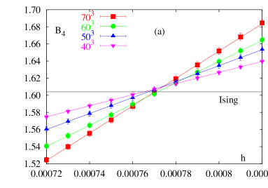
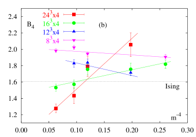
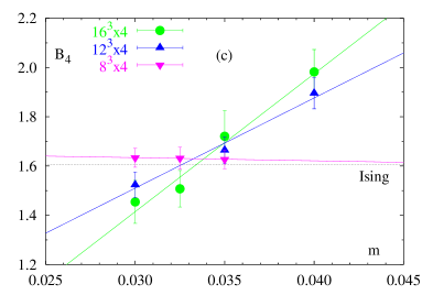
Figure 1: $B_{4,L}$ of the Potts model (a) and for the QCD with heavy (b) resp. light (c) quark masses.(Lines are drawn to guide the eyes)

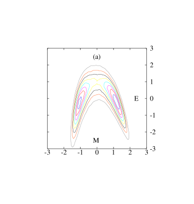
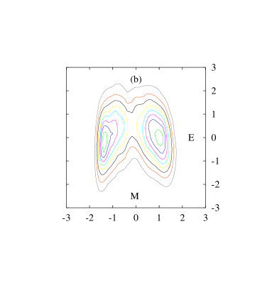
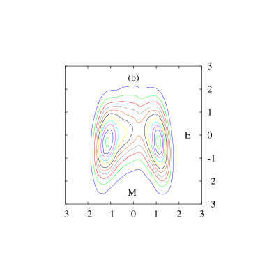
Figure 2: Histogram $\hat{p}_{{\mathcal{E}}{\mathcal{M}}}$ of the Potts model (a) at the endpoint and of the QCD with $m=1.8$ (b), $m=0.325$ (c) close to the end points.

References

- [1] B. Svetitsky, L. Yaffe, Nucl. Phys. B210 (1982) 423.
- [2] F. Karsch, S. Stickan, Phys. Lett. B488 (2000) 319.
- [3] F. Karsch, E. Laermann, Ch. Schmid, hep-lat/0107020
- [4] S. Gavin, A. Gocksch, R.D. Pisarski, Phys. Rev. D 49 (1994) 49.
- [5] J.J. Rehr, N.D. Mermin, Phys. Rev. A 8 (1973) 472.
- [6] N.B. Wilding, A.D. Bruce, J. Phys. Cond. Mat. 4 (1992) 3087.
- [7] A. M. Ferrenberg, R.H. Swendsen, Phys. Rev. Lett. 61 (1988) 2635.