Relativistic Bottomonium Spectrum from Anisotropic Lattices

Abstract

We report on a first relativistic calculation of the quenched bottomonium spectrum from anisotropic lattices. Using a very fine discretisation in the temporal direction we were able to go beyond the non-relativistic approximation and perform a continuum extrapolation of our results from five different lattice spacings ($0.04-0.17$ fm) and two anisotropies (4 and 5). We investigate several systematic errors within the quenched approximation and compare our results with those from non-relativistic simulations.

I INTRODUCTION

The recent experimental activities at B-factories have triggered many theoretical attempts to understand heavy quark phenomenology from first principles. The non-perturbative study of heavy quark systems is complicated by the large separation of momentum scales which are difficult to accommodate on conventional isotropic lattices. These problems are particularly severe in heavy quarkonia, where the small quark velocity separates the high momentum scales around the heavy quark mass from their small kinetic energy; $m_{q}\gg m_{q}v^{2}$. While this motivates the adiabatic approximation and potential models, a full dynamical treatment poses significant computational problems. The limitations of present computer resources force us to tackle this problem in some modified framework. Thankfully there is also a wealth of spectroscopic data against which different lattice methodologies and improvement schemes can be tested. Once experimental results can be understood with some accuracy the lattice will provide a powerful tool for other non-perturbative predictions such as decay rates and form factors involving heavy quarks.

Several approximations to relativistic QCD have been proposed to describe accurately the low energetic phenomenology of heavy quarkonia [1, 2]. However, the (non-)perturbative control of systematic errors in those approximations is very difficult and in practise one has to rely on additional approximations. The high precision results for the spin structure in non-relativistic bottomonium calculations[3] have been hampered by large systematic errors which are difficult to control within this effective theory. Higher order radiative and relativistic corrections are sizeable for bottomonium [4, 5] and even more so for charmonium [6]. Still more cumbersome are large observed scaling violations [6, 7] that cannot be controlled by taking the continuum limit.

We take this as our motivation to study heavy quarkonia on anisotropic lattices in a fully relativistic framework. This approach has previously been used to calculate the charmonium spectrum with unprecedented accuracy [8, 9, 10, 11]. Here we extent the method to even heavier quarks and focus on our new results for bottomonium. Preliminary results were already reported in [10].

There are additional advantages in using anisotropic lattices which have been employed previously. It has been demonstrated by several authors that a fine resolution in the temporal direction is useful in controlling and extracting higher excitations and momenta in the QCD spectrum [12, 13, 14, 15]. It has been noticed long ago that anisotropic lattices are also the natural framework to study QCD at finite temperature [16]. This has been used in [17, 18] to retain more Matsubara frequencies at high temperature. Furthermore, it has been suggested that anisotropic lattices can circumvent problems arising due to unphysical branches of the dispersion relation on highly improved lattices [19].

In Section II we introduce the anisotropic gauge and quark action for our study. In Section III we give the details of our simulation and study systematic errors in Section IV. Our results are discussed in Section V and Section VI concludes this paper.

II Anisotropic Lattice Action

The basic idea of our approach is to control large lattice spacing artifacts from the heavy quark mass by adjusting the temporal lattice spacing, $a_{t}$, such that $m_{q}a_{t}<1$. For the bottomonium system this implies $a_{t}^{-1}>5$ GeV. Discretisation errors from spatial momenta are controlled by $|{\bf p}|a_{s}<1$, which can be satisfied more easily at conventional spatial lattice spacings $a_{s}^{-1}>1.5$ GeV. We retain the isotropy in all the spatial directions. The continuum limit can then be taken at fixed anisotropy, $\xi=a_{s}/a_{t}$.

More specifically, we employ an anisotropic gluon action, which is accurate up to ${\cal O}(a_{s}^{2},a_{t}^{2})$ discretisation errors:

$$S=-\beta\left(\sum_{x,{\rm i>j}}\xi_{0}^{-1}P_{\rm ij}(x)+\sum_{x,{\rm i}}\xi_{0}P_{\rm it}(x)\right)~{}~{}.$$ (1)

This is the standard Wilson action written in terms of simple plaquettes, $P_{\mu\nu}(x)$. Here $(\beta,\xi_{0})$ are two bare parameters, which determine the spatial lattice spacing, $a_{s}$, and the renormalised anisotropy, $\xi$, of the quenched lattice. For the heavy quark propagation in the gluon background we used the “anisotropic clover” formulation as first described in [8, 9]. The discretised form of the continuum Dirac operator, $Q=m_{q}+D\hskip-6.25963pt/$, reads

$$Q = m_{0}+\nu_{t}~{}W_{0}\gamma_{0}+\nu_{s}~{}W_{i}\gamma_{i}-\frac{a_{s}}{2}\left[c_{t}~{}\sigma_{0k}F_{0k}+c_{s}~{}\sigma_{kl}F_{kl}\right]~{}~{},$$ (2)

$$W_{\mu} = \nabla_{\mu}-(a_{\mu}/2)\gamma_{\mu}\Delta_{\mu}~{}~{}.$$ (3)

Here $\nabla_{\mu}$ denotes the symmetric lattice derivative and $a_{\mu}^{2}\Delta_{\mu}q(x)\equiv U_{\mu}(x)~{}q(x+\mu)-2~{}q(x)+U_{-\mu}(x)~{}q(x-\mu)$. For the electromagnetic field tensor $F_{\mu\nu}$ we choose the traceless cloverleaf definition which sums the 4 plaquettes centered at point $x$ in the $(\mu,\nu)$ plane:

$$a_{\mu}a_{\nu}~{}F_{\mu\nu}(x)\equiv\frac{i}{2}\left[P_{\mu\nu}(x)+P_{\nu\bar{\mu}}(x)+P_{\bar{\mu}\bar{\nu}}(x)+P_{\bar{\nu}\mu}(x)-h.c.\right]~{}~{}.$$ (4)

As has been demonstrated by P. Chen [9], Eq. (3) is equivalent to the continuum action (up to ${\cal O}(a^{2})$ errors) through $O(3)$ symmetric field redefinition:

$$q(x)\to\left(1+\frac{\Omega_{m}}{2}a_{t}m_{q}+\frac{\Omega_{t}}{2}a_{t}/\hskip-5.69046pt\nabla_{t}+\frac{\Omega_{s}}{2}a_{s}/\hskip-5.69046pt\nabla_{s}\right)q(x)~{}~{}.$$ (5)

In a recent paper [20], S. Aoki et al. observed that this 5-parameter fermion action does not generate Euclidean $O(4)$ covariant quark propagators. While it is true that the fermion Green’s functions derived from our action will contain non-covariant terms at ${\cal O}(a)$, these can be removed by undoing the field transformation (5) at the end of the calculation. Rather than working with a more complicated action where additional parameters have to be tuned for covariance, it would be easier to implement this change of spinor basis after the expensive inversion of the fermion matrix. However, in this work we do not even need such a final transformation since we do not study spin-1/2 hadrons. We have chosen Wilson’s combination, $W_{\mu}$, of first and second derivative terms so as to ensure the full projection property and to remove all doublers. The five parameters in Eq. (3) are all related to the quark mass, $m_{q}$, and the gauge coupling as they appear in the continuum action. By tuning them appropriately we can remove all ${\cal O}(a)$ errors and re-establish Euclidean $O(4)$ symmetry. The classical estimates have been given in [9]:

$$m_{0} = m_{q}(1+\frac{1}{2}~{}a_{s}m_{q})$$ (6)

$$\nu_{t} = \nu_{s}\frac{1+\frac{1}{2}~{}a_{s}m_{q}}{1+\frac{1}{2}~{}a_{t}m_{q}}$$ (7)

$$c_{s} = \nu_{s}$$ (8)

$$c_{t} = \frac{1}{2}\left(\nu_{s}+\nu_{t}\frac{a_{t}}{a_{s}}\right)~{}~{}.$$ (9)

Simple field rescaling enables us to set one of the above coefficients at will. For convenience we fix $\nu_{s}=1$ and adjust $\nu_{t}$ non-perturbatively for the mesons to obey a relativistic dispersion relation ( $c({\bf 0})=1$ ):

$$E^{2}({\bf p}) = E^{2}({\bf 0})+c^{2}({\bf p})~{}{\bf p}^{2}+{\cal O}({\bf p}^{4})\ldots~{}~{}.$$ (10)

We also chose $m_{0}$ non-perturbatively, such that the rest energy of the hadron matches its experimental value ($M(^{3}S_{1}^{--})$ = 9.46 GeV for bottomonium). For the clover coefficients $(c_{s},c_{t})$ we take their classical estimates from Eqs. (8) and (9) and augment the action by tadpole improvement:

$$U_{i} \to U_{i}/u_{s}$$ (11)

$$U_{0} \to U_{0}/u_{t}~{}~{}.$$ (12)

Following Ref. [9] the resulting (dimensionless) fermion matrix can then be written as

$$a_{t}Q=u_{t}\hat{m}_{0}+\nu_{t}~{}\hat{W}_{0}\gamma_{0}+\frac{\nu_{s}}{\xi_{0}}~{}\hat{W}_{i}\gamma_{i}-\frac{1}{2}\left[\frac{c_{t}}{u_{t}u_{s}^{2}}~{}\sigma_{0k}\hat{F}_{0k}+\frac{c_{s}}{u_{s}^{3}\xi_{0}}~{}\sigma_{kl}\hat{F}_{kl}\right]~{}~{},$$ (13)

where we arranged the terms in such a way that the temporal Wilson term is multiplied by only $\nu_{t}$. To compute the coefficients of the spatial terms we used $\xi/\xi_{0}=u_{t}/u_{s}$, which is accurate within 3% [9, 21]. Remember that we can still choose $\nu_{s}$ at will and a 3% uncertainty for $c_{s}$ is certainly acceptable – at our lattice spacings a different tadpole prescription has a much more pronounced effect on this coefficient. The tadpole coefficients have been determined from the average link in Landau gauge: $u_{\mu}=1/3~{}\langle{\rm tr}~{}U_{\mu}(x)\rangle_{\rm Landau}$. For brevity we will refer to this as the Landau scheme. Any other choice for $(c_{s},c_{t})$ will have the same continuum limit, but with this prescription we expect only small ${\cal O}(\alpha a)$ discretisation errors.

III Simulation Details

For the generation of quenched gauge field configurations we employ a standard heat-bath algorithm as it is also used for isotropic lattices. The renormalised anisotropy, $\xi$, is related to the bare parameter $\xi_{0}$ through:

$$\xi=\eta(\xi,\beta)~{}\xi_{0}~{}~{}.$$ (14)

A convenient parametrisation for $\eta$ can be motivated by a one-loop analysis of the renormalised anisotropy:

$$\eta(\xi,\beta)=1+(1-\frac{1}{\xi})~{}\frac{\hat{\eta}_{1}(\xi)}{\beta}~{}\frac{1-a_{1}~{}g^{2}}{1-a_{0}~{}g^{2}}~{}~{},$$ (15)

where $\hat{\eta}_{1}(\xi)\approx 1.02$ and almost constant for our range of $\xi$. We use Padé parameters ($a_{0}=-0.77810$ and $a_{1}=-0.55055$) which have been determined by an excellent fit over a wide range of lattice data with different $\beta$ and $\xi$ [21]. Based on Eq.15 we choose the appropriate $\xi_{0}$ to realize $\xi$ close to 4 and 5 for each value of $\beta=6/g^{2}=5.7-6.5$ . Depending on the gauge coupling, we measure hadron propagators every 100-400 sweeps in the update process, which is sufficiently long for the lattices to decorrelate.

The construction of meson operators with given $J^{PC}$ assignment is standard. As in Refs.[10, 22], we use both local and extended operators by employing the 16 $\Gamma$-matrices and spatial lattice derivatives for the quark-bilinears:

$$M(x)=\bar{q}(x)\Gamma_{i}\Delta_{j}[U]\Delta_{k}[U]q(x)~{}~{}.$$ (16)

To improve the overlap with the ground state we also implemented a combination of various iterative smearing prescriptions for the quark fields and gauge links:

$$q(x) \to q^{(n)}(x)=(1-\frac{\epsilon}{n}\Delta^{2}[U])^{n}q(x)\mbox{\hskip 99.58464pt\it Jacobi smearing}$$ (17)

$$U(x) \to U^{(m+1)}(x)={\cal P}_{SU(3)}~{}\left(U^{(m)}(x)+\alpha\sum_{\rm staples}S(x)\right)\mbox{\it~{}~{}~{}~{}~{}APE smearing}$$ (18)

For conventional states, we find it often sufficient to use (gauge-fixed) box sources of different size. We use local sinks throughout. This setup allows us to extract reliably both the ground state energies and their excitations from correlated multi-state fits to several smeared correlators, $C^{s}(t)$, with the same $J^{PC}$:

$$C^{s}(t,{\bf p})\equiv\langle M(t,{\bf p})~{}M^{s}(0,{\bf p})\rangle=\sum_{i=1}^{\rm n_{fit}}~{}a_{i}^{s}({\bf p})~{}\left(e^{-E_{i}({\bf p})~{}t}+e^{-E_{i}({\bf p})(N_{t}-t)}\right)~{}~{}.$$ (19)

Since we are working in a relativistic setting, the second term takes into account the backward propagating piece from the temporal boundary. An example of this is given in Figure 1, where we show the effective masses for ${{}^{3}S}_{1}=1^{--}$ from three different box sources along with the fit results from a 2-state and 3-state ansatz. In this example the smallest box shows clear contributions from excited states, while the other two sources project much better onto the ground state. We did not further optimize the box size for perfect overlap, but since for the largest source the plateau is approached from below we can estimate that an “optimal” box would have a physical extent of 0.2-0.3 fm. This is in good agreement with phenomenological expectations about the size of the $\Upsilon$ ground state. What is more important here for us is to have a variety of different overlaps which are well suited to constrain the multi-state fits.

To obtain the dispersion relation, $E({\bf p})$, we project the meson correlator also onto four different non-zero momenta by inserting the appropriate phase factors, $\exp{(-i{\bf px})}$, at the sink. This is illustrated in Figure 2, where we use

$${\bf p}=\left(\frac{2\pi}{N_{s}}\right)~{}{\bf n}\hskip 28.45274pt\mbox{with~{}~{}~{}}{\bf n}=(0,0,0),(1,0,0),(1,1,0),(2,0,0),(2,2,0)~{}~{}.$$ (20)

For an estimate of the spin-splittings we take the difference of the ground state masses from multi-state fits. Because these states are highly correlated we obtain very accurate estimates for the spin-splittings compared to the absolute masses. An example of this is shown in Figure 3. We use jackknife and bootstrap ensembles for our error estimates and find good agreement in all cases. In order to call a fit acceptable we require consistency within errors for different fit ranges and Q-values to be bigger than 0.1. Our main results are collected in Table I along with the input parameters for the different data sets.

For $(\beta,\xi)=(6.1,4)$ and $(6.3,4)$ we have also analyzed extended operators that give access to $2^{++}={{}^{3}}P_{2}$, $D$-states with two units of orbital angular momentum and exotic hybrid states, Table II. These are more states than previously obtained from non-relativistic calculations. Even though our scaling window is not wide enough to make a serious attempt of a continuum extrapolation, we expect lattice artifacts to be less pronounced for those large states. At (6.1,4) we find a good agreement of our results and those reported in [13, 14, 22]. This is not unexpected since the non-relativistic approximation is known to work better for hybrid states, which are thought to live in a very shallow potential [14]. In particular we find the lowest lying hybrid to be the $1^{-+}$. We are however concerned that these results are more sensitive to finite volume effects than those for $S$ and $P$ states, see Sec. IV. Especially at (6.3,4) we have reason to believe that our lattice is not sufficiently big to accommodate such large wavefunctions, resulting in an inversion of the characteristic level ordering. A simulation on bigger volumes is necessary to simulate hybrid states more accurately.

In the following we will focus on the low-lying bottomonium states and their spin-structure where statistical errors are small enough to allow a critical comparison with results from the non-relativistic approximation.

IV Systematic errors

Apart from our main data sets we performed extensive checks of systematic errors within the quenched approximation. As mentioned above, we enforce a relativistic dispersion relation by tuning the bare parameter $\nu_{t}$ non-perturbatively at each quark mass to obtain c=1.0 very accurately within $1-2\%$. From a classical analysis of the dispersion relation we expect $c\propto 1/\nu_{t}$. Indeed, for an arbitrary decrease of $\nu_{t}$ by $10\%$ we observe an increase of the velocity of light by a similar amount (7.8(2.1)%), see Table III and Figure 4. Within the statistical error for the P structure we could not resolve any significant effect, while the hyperfine splitting showed an increase by $8(10)\%$. From those observations, we expect only small changes ($<2\%$, $<1$ MeV) due to $c\neq 1$.

We also tested for finite size effects by explicitly comparing the results from two different spatial volumes of $(1.3\mbox{~{}fm})^{3}$ and $(0.7\mbox{~{}fm})^{3}$ at $(\beta,\xi)=(6.1,4)$, see Figure 5. While changes in the ground state masses amount to only a fraction of a percent, the hyperfine splitting shows a slight increase of 6(4)% and the ${{}^{1}P}_{1}-{{}^{3}S}_{1}$ splitting is reduced by 10(9)% when going to the larger lattice. Therefore we expect the hyperfine splitting to be systematically underestimated when $L<1$ fm. For the fine structure we could not resolve any shift within the statistical errors. For all but our finest lattice we have $L\approx 1$ fm which should be sufficiently big to accommodate the small bottomonium ground states in a quenched simulation.

Another source of systematic errors is the tuning of the bare quark mass parameter, $m_{0}$. Especially for the hyperfine splitting we observed a strong dependence on the ground state mass, $M(m_{0})$, as shown in Figure 6. On our coarser lattices we were able to tune the mass very accurately to within 10% of the physical bottomonium mass, but as the tuning becomes more and more expensive on our finer lattices, the deviation from bottomonium reaches 35(15)% at $(\beta,\xi)=(6.5,4)$. We use the potential model prediction, $\Delta E_{\rm hfs}\propto 1/M$, to rescale all measured $\Delta E_{\rm hfs}$ to the physical point, $M=9.46$ GeV. Our results in Table I include these adjustments in both the central values and their errors. Since all spin splittings vanish in the static limit we also apply the same rescaling technique to the fine structure.

Finally there will be systematic effects at finite lattice spacing, which are absent in the continuum limit. The tree-level estimates for $c_{s}$ and $c_{t}$ will experience a shift due to radiative corrections, thereby changing the magnitude of the ${\cal O}(\alpha a)$ artifacts. In Figure 7 and Table IV we compare the Landau scheme with another popular scheme, where the tadpole coefficients are estimated from the plaquette values: $3u_{\mu}=\langle{\rm tr}~{}P_{i\mu}\rangle^{1/4}$. This amounts to a $(10\%,2\%)$ change in $(c_{s},c_{t})$ at (5.9, 4). The corresponding change in the hyperfine splitting is -15(17)%. While this may indicate some additional reduction at coarse lattices (resulting in a slightly worse scaling behaviour), it is also clear that within our errors we are not very sensitive to this choice of tadpole coefficients. Since any remaining difference will vanish in the continuum limit we did not investigate this dependence further.

V Discussion

To convert lattice data into dimensionful quantities we used the lattice spacing determined from the ${{}^{1}P}_{1}-{{}^{3}S}_{1}$ splitting which is fixed to match the experimental value ($\approx 440$ MeV). It is well-known that, without dynamical sea quarks in the gluon background, the definition of the lattice spacing is ambiguous and one cannot reproduce all experimental splittings simultaneously. Non-relativistic lattice calculations with two dynamical flavours [5, 7] resulted in shifts of up to 5 MeV for the hyperfine splitting, but they are also not completely free from ambiguities in the lattice spacing and from systematic errors such as lattice spacing artifacts, radiative and relativistic corrections. For the purpose of this paper we accept the shortcomings of the quenched approximation and aim to control the other systematic errors instead, the combined effect of which could also be as large as 20% for bottomonium on the lattices in this study.

The main features of the bottomonium spectrum from relativistic lattice QCD are summarised in Figure 8, where we can see clearly the characteristic level ordering as additional angular momentum is inserted into the ground state. The overall agreement with experimental data is impressive, as is the spin-structure predicted from first principles. While it is probably too early to investigate the spin-splittings in excited states ($2~{}{{}^{3}S}_{1}-2~{}{{}^{1}}S_{0}$ has still large statistical errors), we have rather accurate data for the spin-structure of the ground states.

In Figure 9 we plot the hyperfine splitting against the spatial lattice spacing at fixed anisotropy and compare it with previous simulations in this region. Already at finite lattice spacing we can see significant deviation from non-relativistic simulations. There could be several reasons for this. First, we should expect different discretisation errors from the different gluonic actions that have been employed in the past. While the unquenched results in Figure 9 were obtained from an RG-improved gluon action with two dynamical flavours [7], many other quenched simulations where done using the standard plaquette action [3, 4, 5, 23]. Non-relativistic results from coarse and anisotropic lattices also exist [24] and they seem to show scaling violations similar to those from unimproved gluon actions, even though a plaquette-plus-rectangle (Symanzik) action had been used. This could be an indication of comparatively large ${\cal O}(\alpha a)$ corrections which can compete with ${\cal O}(a^{2})$.

Some of those results mentioned also use a different prescription for the tadpole coefficients than in our present work. We want to stress again that the tadpole prescription is merely an empirical way of keeping radiative corrections small. It has been suggested by several authors that the Landau scheme is particularly suitable to account for radiative corrections due to tadpole diagrams [6, 25]. In the continuum limit ($U_{\mu}\to 1$) both definitions (Landau and plaquette) will be identical, but at finite lattice spacing they result in different estimates for the clover coefficients. We have demonstrated above that a lower value for $u_{0}$ will result in a slightly larger hyperfine splitting. A more pronounced effect has been observed in [5]. In the non-relativistic framework one can also quantify this shift which has been employed in [23]. These authors rescale their results to the Landau scheme and found improved scaling. Here we find some indication for a minor improvement, but none of the schemes is completely successful in removing the apparently large ${\cal O}(\alpha a)$ errors. A non-perturbative determination of the clover coefficients is in order to reduce those errors significantly. We used the Landau scheme mainly for simplicity.

In contrast, the fine-structure is not expected to be as much affected by the tadpole prescription which can explain the better agreement of our estimates for ${{}^{3}P}_{1}-{{}^{3}P}_{0}$ with the NRQCD values in Figure 10.

We interpret the remaining differences between our results and the quenched NRQCD values as due to higher order relativistic effects. It has already been shown in [4, 5] that those corrections can be sizable ($>10\%$ for bottomonium at ${\cal O}(mv^{6})$). However, it is not trivial to extend the non-relativistic approximation to ever higher order. Our calculation does not suffer from this uncertainty since we are working in a fully relativistic setting.

Above all we are now able to perform a continuum extrapolation of the hyperfine splitting. As shown in Figure 9 the scaling violations are large and we parameterise our lattice results by 1) a linear ansatz, 2) by a quadratic ansatz and 3) by a linear-plus-quadratic fit in $a_{s}$. All these fits are acceptable with $Q=0.3\ldots 0.9$. For the final analysis we also decided to omit the results from our coarsest lattice where we should expect potentially large lattice spacing corrections from higher orders due to $a_{t}m_{q}>1$ and $a_{s}m_{q}v>1$. Including this data, however, does not change our continuum estimates significantly. If we assume that our action successfully removes all ${\cal O}(a)$ errors, we can quote 51.1(3.1) MeV for the quenched hyperfine splitting in bottomonium. This may be too optimistic and, allowing for ${\cal O}(\alpha a)$ errors, we find 59(20) MeV from a linear-plus-quadratic fit. As can already be seen from the large error on the intercept, such a general fit is not very well constrained by our data and even the quadratic term is consistent with zero. For comparison, we find 58.7(5.5) MeV from a simple linear fit. Notice though, that all these fitting methods result in comparatively high values given phenomenological estimates of 30-40 MeV. It remains to be seen how unquenching will affect this quantity, although we expect that it would further increase the hyperfine splitting. An accurate experimental determination of the bottomonium hyperfine splitting would be most valuable to judge the reliability of our approach.

For the fine structure, ${{}^{3}P}_{1}-{{}^{3}P}_{0}$, the situation is very similar as shown in Figure 10. We find a rather large value of 50.9(6.4) MeV from the simple linear extrapolation in $a_{s}$ ($Q=0.22$). This is $3\sigma$ above the experimental value of 32.1(1.5) MeV. The quadratic fit is slightly worse ($Q=0.14$) and predicts 41.7(4.1) MeV for the continuum limit. As for the hyperfine splitting, a fit involving both terms is badly constrained and gives 68(22) MeV with $Q=0.12$.

In Figure 11 we also plot the higher excitation, $2S-1S$, against the spatial lattice spacing. Naturally these results have larger errors than spin-splittings and ground states as they rely on the control of additional parameters (amplitudes and energies) in the fitting process. In line with other simulations, we find a continuum result which is slightly larger than the experimental value. However, it will be important to measure this quantity more accurately on bigger volumes as our lattices may not be big enough for those larger states. Based on the observed finite volume effects, Figure 5, we have reason to believe that the result from our finest lattice $(\beta,\xi)=(6.5,5)$ could be overestimated. Therefore we treat our data for the $2S-1S$ splitting with caution.

VI Conclusion

In conclusion, we have demonstrated that also systems containing quarks as heavy as bottom can be treated relativistically within the framework of anisotropic lattice QCD. Imposing a fine temporal discretisation appears to be a very natural way to respect the physical scales in the problem and it should open up a reliable alternative to non-relativistic simulations (where systematic errors are much harder to control). In our study of the bottomonium system we found noticeable deviations of the hyperfine splitting from non-relativistic simulations, while the fine-structure agrees well with previous results. Overall we observed strong scaling violations resulting in a relatively large value and large errors for the continuum limit. This however, is not totally unexpected as we only used a tree-level estimate for the clover coefficients and did not tune them non-perturbatively to eliminate ${\cal O}(a_{s})$ effects completely. We believe that further studies on anisotropic lattices will be able to determine the continuum spectrum of bottomonium with increasing accuracy. A non-perturbative determination of the clover coefficients is highly desirable, but it remains to be seen whether this is feasible as suggested in [26]. Alternatively, simulations at even finer lattice spacings would be useful to disentangle remaining ${\cal O}(a_{s})$ and ${\cal O}(a_{s}^{2})$ errors. What remains to be done is the efficient implementation of anisotropic sea quarks which is necessary to control the systematic errors from the quenched calculation. Work in this area is in progress [27].

Future applications are not restricted to heavy quark masses alone, but they may also be extended to heavy-light systems where both quarks can now be treated within a uniform approach.

Acknowledgments

This work was conducted on the QCDSP machines at Columbia University and RIKEN-BNL Research Center. We like to thank N. Christ and R. Mawhinney for their valuable comments and suggestions. TM and XL are supported by the U.S. Department of Energy.

$(\beta,\xi)$	(5.7,4)	(5.9,4)	(5.9,5)	(6.1, 4)	(6.1, 4)	(6.1, 5)	(6.3 ,4)	(6.5 ,4)
$(N_{s},N_{t})$	(8, 96)	(8, 96)	(8, 96)	(16,96)	(8,96)	(16,128)	(16,128)	(16,160)
configs	392	700	780	660	420	370	450	710
separation	100	100	400	400	400	400	400	400
$a_{t}^{-1}$ [GeV]	4.54(31)	6.76(24)	9.27(43)	10.57(31)	9.65(75)	12.3(1.2)	15.15(81)	20.9(2.2)
$a_{s}$ [fm]	0.174(12)	0.1168(42)	0.1064(49)	0.0747(22)	0.0818(64)	0.0804(77)	0.0521(28)	0.0377(40)
$\xi_{0}$	3.04682	3.139035	3.870249	3.210801	3.210801	3.96234	3.268645	3.31655
$u_{0s}$	0.758364	0.785945	0.784067	0.800927	0.800927	0.81015	0.826810	0.83709
$u_{0t}$	0.984104	0.986984	0.991782	0.988702	0.988702	0.99279	0.990039	0.99100
$u_{0t}/u_{0s}$	1.297667	1.255793	1.26492	1.234447	1.234447	1.22544	1.197420	1.18386
$\xi/\xi_{0}$	1.312844	1.274277	1.2919065	1.245795	1.245795	1.26188	1.223749	1.20607
$a_{t}m_{q}$	1.98	1.1200	0.8960	0.6700	0.6700	0.58	0.4940	0.31
($\nu_{s},\nu_{t}$)	(1, 1.30)	(1, 1.50)	(1, 1.815)	(1, 1.573)	(1, 1.573)	(1,1.65)	(1, 1.5)	(1,1.51)
$c_{s}$	2.292804	2.059794	2.074632	1.946351	1.946351	1.88063	1.7680	1.7054
$c_{t}$	1.170549	1.127661	1.1177481	1.098368	1.098368	1.05055	1.0154	0.9002
$c(0)$	1.044(25)	1.026(32)	0.990(11)	0.979(7)	1.018(14)	0.994(11)	1.004(19)	0.992(20)
${{}^{3}}S_{1}$ [GeV]	9.79(66)	9.53(34)	9.57(44)	10.40(30)	9.49(74)	10.11(97)	12.60(67)	13.04(14)
1 ${{}^{3}}S_{1}-{{}^{1}}S_{0}$ [MeV]	36.0(3.5)	37.2(2.6)	37.5(2.9)	44.8(2.0)	33.8(3.1)	37.0(5.7)	49.9(4.9)	51.0(7.9)
2 ${{}^{3}}S_{1}-{{}^{1}}S_{0}$ [MeV]	155(273)	56(57)	37(12)	40(11)	57(18)	2(58)	48(41)	57(29)
${{}^{1}}P_{1}-{{}^{3}}P_{0}$ [MeV]	16.2(4.7)	20.6(4.5)	25.2(3.2)	39.5(5.7)	28.7(6.6)	30.7(5.5)	54.0(7.7)	46.6(8.7)
${{}^{1}}P_{1}-{{}^{3}}P_{1}$ [MeV]	-1.4(2.3)	-1.3(1.1)	4.6(1.3)	8.0(3.3)	7.9(4.9)	3.7(2.0)	8.8(3.5)	8.4(3.8)
${{}^{3}}P_{1}-{{}^{3}}P_{0}$ [MeV]	16.0(2.8)	23.7(3.1)	24.5(2.2)	28.3(4.0)	28.0(5.7)	27.4(4.2)	44.7(5.1)	39.9(6.6)
$R_{2S}$	1.00(23)	1.37(18)	1.40(14)	1.27(14)	1.38(17)	1.30(25)	1.53(18)	1.53(20)
$R_{3S}$	1.99(50)*	2.35(29)*	3.13(32)*	2.27(34)*	3.6(1.3)*	3.05(57)*	3.25(51)*	5.17(76)*
$R_{2P}$	2.21(48)*	2.32(30)	2.26(26)	2.40(13)	2.26(30)	1.98(61)	2.56(49)	2.14(34)

TABLE I.: Simulation Parameters and Results. We label our runs by $(\beta,\xi)$, where $\beta$ is chosen to vary the spatial lattice spacing and $\xi$ determines the appropriate bare anisotropy $\xi_{0}$, see Eq. 15. The temporal lattice spacing, $a_{t}$, is determined from ${{}^{1}}P_{1}-{{}^{3}}S_{1}$. Ground state and higher excitations are from correlated 3-cosh fits to all channels. For the excitations we quote their normalized results $R_{X}\equiv(X-1S)/(1P-1S)$. An asterisk denotes results which have not been checked by fitting even higher excitations than those listed. For example, we did not perform 4-cosh fits to obtain better estimates for $3S$. All spin-splittings have been rescaled to the physical bottomonium (${{}^{3}S}_{1}=9.46$ GeV).

$(\beta,\xi)$	(6.1, 4)	(6.3 ,4)
configs	330	360
separation	400	400
${{}^{3}}P_{2}-{{}^{1}}P_{1}$ [MeV]	24.4(4.1)	20.6(6.9)
${{}^{3}}P_{2}-{{}^{3}}P_{1}$ [MeV]	39(14)	27(11)
$2^{--}-2^{-+}$ [MeV]	–	31.0(6.9)
$R_{2^{-+}}$	–	1.63(11)
$R_{2^{--}}$	1.81(26)	1.67(11)
$R_{1^{-+}}$	3.41(43)	4.25(34)
$R_{0^{+-}}$	4.41(85)	3.37(72)
$R_{2^{+-}}$	–	5.93(45)

TABLE II.: Results from extended meson operators. For the two lattices shown all run parameters are exactly as in Table I and $R_{X}$ is the normalized excitation above the ground state: $R_{X}\equiv(X-1S)/(1P-1S)$. However, here we employ also the extended operators of Eq. (16) which give us access to ${{}^{3}P}_{2}$, states with $L=2$ and the exotic hybrid candidates $(0^{+-},1^{-+},2^{+-})$. For P-states ($L=1$) we use a single symmetric lattice derivative to create extended operators and for D-states we take the anticommutator $\{\Delta_{i},\Delta_{j}\}$, ($L=2$). The commutator $[\Delta_{i},\Delta_{j}]$ amounts to an insertion of a colour-magnetic field into the quark bilinear and gives rise to hybrid states. Different Dirac matrices result in different $J^{PC}$ assignments.

$(\nu_{s},\nu_{t})$	(1., 1.815)	(1.,1.650)
$(c_{s},c_{t})$	(2.074632, 1.1177481)	(2.074632, 1.090685 )
configs	780	500
$c(0)$	0.990(11)	1.067(18)
$a_{t}^{-1}$ [GeV]	9.27(43)	8.20(34)
${{}^{3}}S_{1}$ [GeV]	9.57(44)	9.05(38)
${{}^{3}}S_{1}-{{}^{1}}S_{0}$ [MeV]	37.5(2.9)	34.4(2.6)
${{}^{1}}P_{1}-{{}^{3}}P_{0}$ [MeV]	25.2(3.2)	24.3(5.7)
${{}^{1}}P_{1}-{{}^{3}}P_{1}$ [MeV]	4.6(1.3)	4.6(1.4)
${{}^{3}}P_{1}-{{}^{3}}P_{0}$ [MeV]	24.5(2.2)	24.6(2.5)
$R_{2S}$	1.40(14)	1.324(81)
$R_{2P}$	2.26(26)	2.54(23)

TABLE III.: Change in $\nu_{t}$. In this table we comapre our results from $(\beta,\xi)=(5.9,5)$ when the optimal $\nu_{t}=1.815$ is changed arbitrarily by 10%. This entails a change in $c_{t}$. All other run parameters are as in column 4 of Tab. I. The corresponding changes in the spectrum as listed above and the lattice numbers are given in Fig. 4.

tadpole scheme	$u_{0L}$	$u_{0P}$	$u_{0L}$	$u_{0P}$
$(\beta,\xi)$	(5.9,4)	(5.9,4)	(6.1, 4)	(6.1, 4)
$(N_{s},N_{t})$	(8, 64)	(8, 64)	(16, 96)	(16, 96)
configs	600	600	660	130
$a_{t}^{-1}$ [GeV]	6.57(43)	6.40(53)	10.57(31)	10.6(1.1)
$a_{s}$ [fm]	0.1202(80)	0.123(10)	0.0747(22)	0.0745(77)
$\xi_{0}$	3.139035	3.139035	3.210801	3.210801
$u_{0s}$	0.785945	0.810698	0.800927	0.822785
$u_{0t}$	0.986984	0.949731	0.988702	0.952954
$a_{s}m_{q}$	1.1200	1.1200	0.6700	0.877
$(\nu_{s},\nu_{t})$	(1.,1.50)	(1.,1.50)	(1.,1.573)	(1.,1.573)
$c_{s}$	2.059794	1.876818	1.946351	1.795316
$c_{t}$	1.127661	1.101421	1.098368	1.079827
$c(0)$	1.014(15)	1.023(14)	0.979(7)	–
${{}^{3}}S_{1}$ [GeV]	9.25(61)	9.04(75)	10.40(30)	12.3(1.3)
${{}^{3}}S_{1}-{{}^{1}}S_{0}$ [MeV]	35.1(3.9)	30.6(3.6)	44.8(2.0)	43.7(6.6)
${{}^{1}}P_{1}-{{}^{3}}P_{0}$ [MeV]	26.0(3.9)	25.0(4.0)	39.5(5.7)	41(14)
${{}^{1}}P_{1}-{{}^{3}}P_{1}$ [MeV]	1.3(1.7)	1.7(2.3)	8.0(3.3)	9.6(8.2)
${{}^{3}}P_{1}-{{}^{3}}P_{0}$ [MeV]	23.7(2.7)	22.3(2.8)	28.3(4.0)	30.8(9.4)
$R_{2S}$	1.45(13)	1.41(13)	1.27(14)	1.37(23)*
$R_{2P}$	2.22(49)	1.81(28)	2.40(13)	3.14(97)*

TABLE IV.: Here we compare our results from different tadpole descriptions at two different lattices spacings. We distinguish between the Landau scheme, $u_{0L}$, as defined in Section II and the plaquette scheme, $u_{0P}$, for which $3u_{\mu}=\langle{\rm tr}~{}P_{i\mu}\rangle^{1/4}$. While there is some indication that the hyperfine splitting increases when $u_{0}$ is decreased at finite lattice spacing, there is no clear improvement of scaling. See discussion in main text.

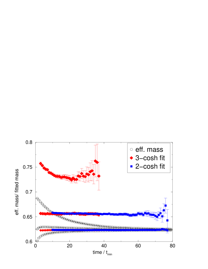
FIG. 1.: Effective masses and fit results. We show the effective masses, open circles, for ${{}^{3}}S_{1}$ at $(\beta,\xi)=(6.5,4)$ from 3 different box sources with spatial extent of 3, 6 and 9 in lattice units. The two larger sources project better onto the ground state as expected. The results from the 2-state and 3-state fits are also shown as filled squares and diamonds, respectively. We observe stable fit results for large enough $t_{\rm min}$. In this example, we fix $t_{\rm max}=80$.

FIG. 2.: Dispersion relation. On the left-hand side we show $t_{\rm min}$-plots for the fitted energy difference between non-zero momentum states and the ${{}^{3}S}_{1}$ at rest. On the right hand side we plot the fitted splitting against the spatial momenta squared, ${\bf p}^{2}=(2\pi/L)^{2}~{}{\bf n}^{2}$. Since we tuned $\nu_{t}$ very carefully, this correspndis to a velocity of light $c(0)=0.990(11)$. This example is from $(\beta,\xi)=(5.9,5)$ with $\nu_{t}=1.815$.

FIG. 3.: Here we show fit results for the ${{}^{3}}P_{1}-{{}^{3}P}_{0}$ splitting at $(\beta,\xi)=(6.1,4),16^{3}\times 96$. We fix $t_{\rm max}=48$ and vary $t_{\min}$ in search for a plateau. Strong correlations between the the two states allow a very accurate determination of the energy difference.

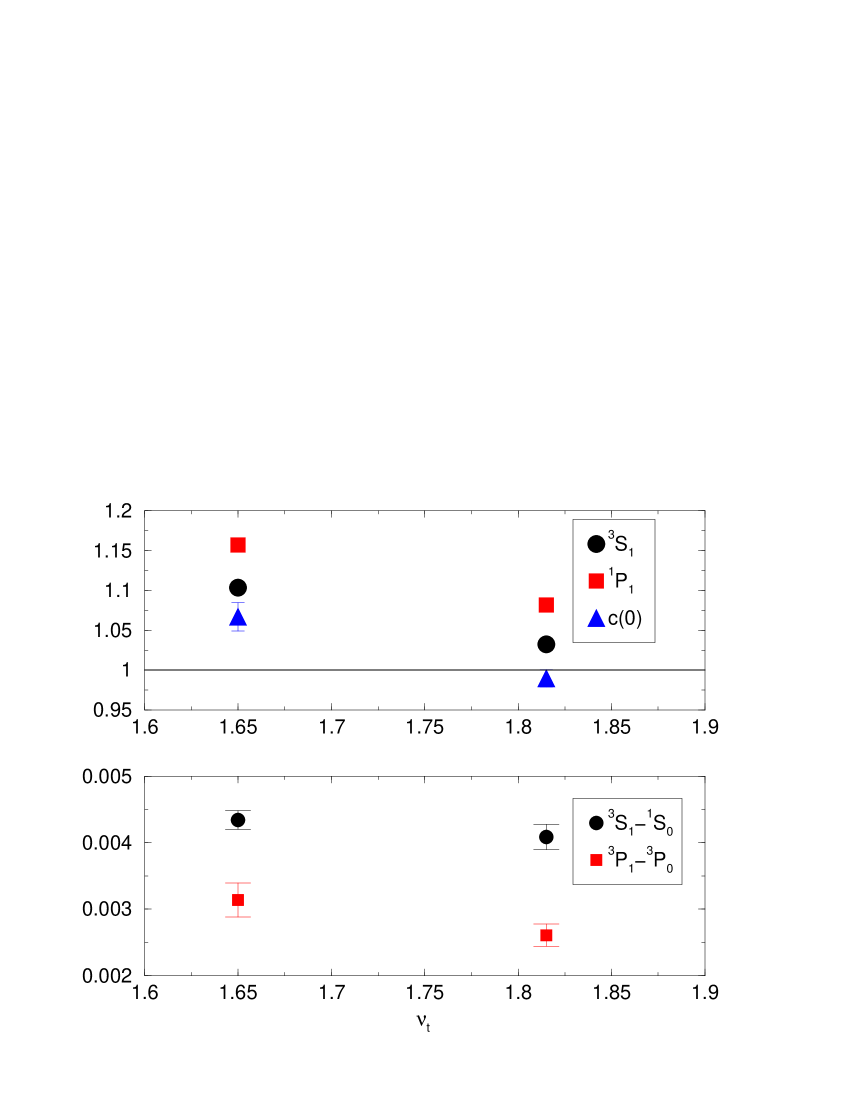
FIG. 4.: $\nu_{t}$-tuning. We illustrate the non-perturbative tuning of the velocity light $(\beta,\xi)=(5.9,5)$. Our best estimate is $\nu_{t}=1.815$ and we show the effect on spectral qunatities as we change this parameter by 10%.

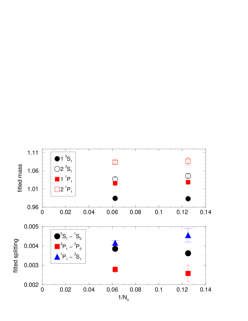
FIG. 5.: Finite volume effects. Here we compare our spectrum results at $(\beta,\xi)=(6.1,4),N_{s}^{3}\times 96$ for $N_{s}=8$ and $16$.

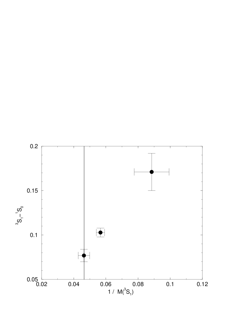
FIG. 6.: Mass dependence. We plot the dimensionless hyperfine splitting against the inverse of the measured meson mass. The vertical line denotes the Bottomonium mass at $(\beta,\xi)=(6.1,4)$. The corresponding bare quark masses are $m_{0}=0.67,0.40$ and $0.10$.

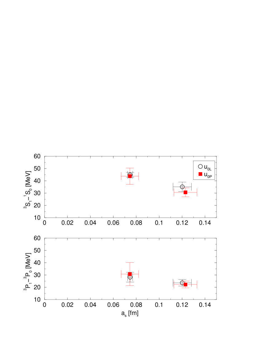
FIG. 7.: Different tadpole prescriptions. Here we compare the effect of changing the value of $(c_{s},c_{t})$ by (10%,2%). Within our statistical errors there is only a minor shift to indicate the corresponding change in ${\cal O}(\alpha a)$ scaling violations.

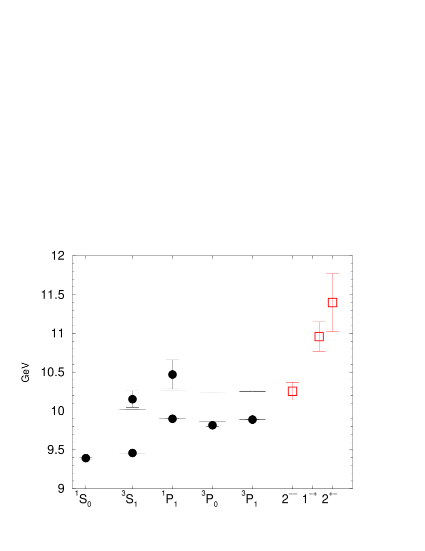
FIG. 8.: Relativistic bottomonium spectrum. We plot our quenched continuum estimates as full circles. Selected results for $2^{--}$ and exotic candidates (hybrids) from finite lattice spacing, (6.1,4), are shown as open squares. The ${{}^{1}P}_{1}-{{}^{3}S}_{1}$ splitting is used to set the scale. Where available, experimental values are shown as horizontal lines.

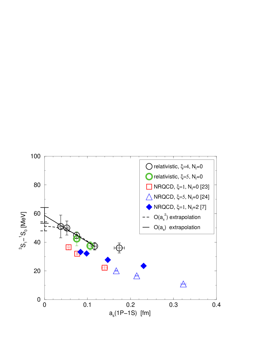
FIG. 9.: Continuum extrapolation of the hyperfine splitting in Bottomonium. Circles denote our results from different anisotropic lattices. Open squares and triangles are quenched NRQCD results from isotropic and anisotropic lattices. Filled diamonds are unquenced NRQCD results with two dynamical flavours at $m_{\pi}/m_{\rho}\approx 0.5$. We also show two different continuum extrapolations of our $\xi=4$ results, where we assume a simple linear or quadratic form in $a_{s}$. The latter results in a better fit but larger continuum value.

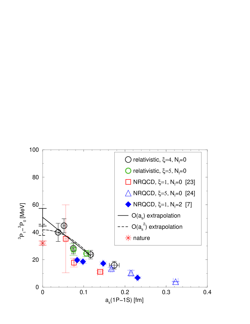
FIG. 10.: Continuum extrapolation of ${{}^{3}P}_{1}-{{}^{3}P}_{0}$. We use the same symbols as in Figure 9 to plot this element of the fine structure against the spatial lattice spacing determined from $1P-1S$.

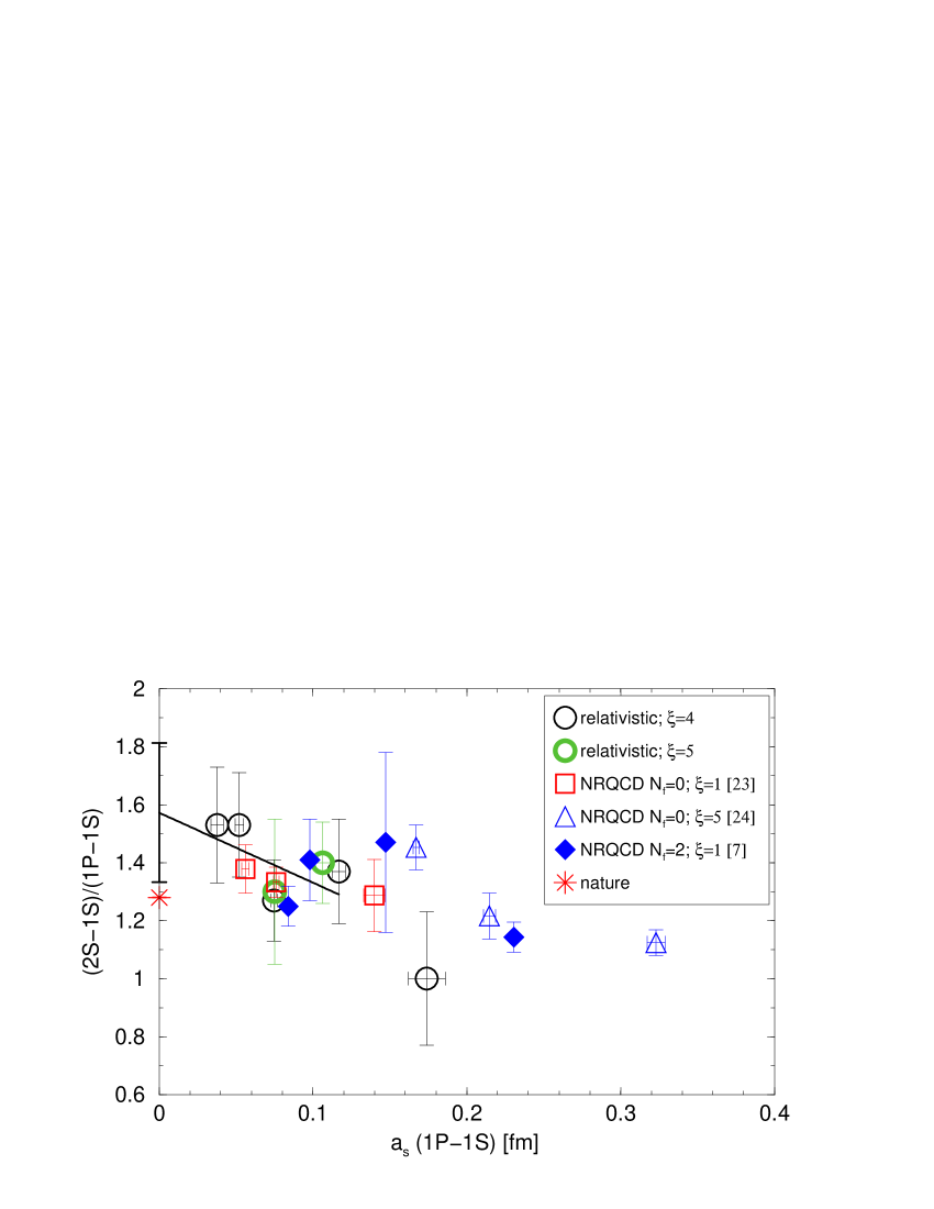
FIG. 11.: Higher excitation in bottomonium, $\Upsilon^{\prime}$. Here we plot the conveniently normalised splitting, $2S-1S$, against the spatial lattice spacing. Within the errors we find a good agreement for all different methods and a slightly higher continuum limit than experiment. From potential models, we can expect that this ratio will be lower in dynamical simulations.

REFERENCES

- [1] B. Thacker and G.P. Lepage, Phys.Rev.D43, 196 (1991); G.P. Lepage et al., Phys.Rev.D46, 4052 (1992).
- [2] A.X. El-Khadra et al., Phys.Rev.D55,3933 (1997); A.X. El-Khadra, Nucl. Phys. B (Proc. Suppl.) 30, 449 (1993).
- [3] C.T.H. Davies et al., Phys. Rev. D50, 6963 (1994).
- [4] T. Manke et al., Phys. Lett.B408, 308 (1997).
- [5] N. Eicker et al., Phys. Rev.D57, 4080 (1998).
- [6] H.D. Trottier, Phys.Rev. D55, 6844, (1997).
- [7] T. Manke et al. (CP-PACS Collaboration), Phys.Rev.D62, 114508 (2000).
- [8] T.R. Klassen, Nucl.Phys. B (Proc.Suppl.) 73, 918 (1999)
- [9] P. Chen, Phys.Rev. D64, 034509, (2001).
- [10] P. Chen et al., Nucl.Phys. (Proc.Suppl.) 94, 342, (2001).
- [11] A. A. Khan et al. (CP-PACS Collaboration), Nucl.Phys.Proc.Suppl. 94, 325, (2001).
- [12] C.J. Morningstar and M. Peardon, Phys.Rev. D56 (1997) 4043.
- [13] T. Manke et al. (CP-PACS Collaboration), Phys.Re v.Lett.82, 4396, (1999).
- [14] K.J. Juge, Phys.Rev.Lett. 82, 4400, (1999).
- [15] S. Collins et al., Phys.Rev. D64, 055002, (2001).
- [16] F. Karsch, Nucl.Phys.B205, 285, (1982).
- [17] Ph. de Forcrand et al. Phys.Rev.D63, 054501, (2001).
- [18] Y. Namekawa et al. (CP-PACS Collaboration), Phys.Rev.D64, 074507, (2001).
- [19] M.G. Alford et al., Nucl.Phys.B496, 377, (1997).
- [20] S. Aoki et al., hep-lat/0107009.
- [21] T.R. Klassen, Nucl.Phys. B 533, 557, (1998).
- [22] T. Manke et al. (UKQCD Collaboration), Phys.Rev. D57, 3829, (1998).
- [23] C.T.H. Davies, et al., Phys.Rev.D58, 054505, (1998).
- [24] T. Manke et al. (CP-PACS Collaboration), Nucl.Phys. (Proc.Suppl.) 86, 397 (2000).
- [25] P. Lepage, Nucl.Phys. (Proc.Suppl.) 60A, 267, (1998).
- [26] T.R. Klassen, Nucl. Phys. B509, 391 (1998).
- [27] L. Levkova and T. Manke, (Proceedings of Lattice 2001), hep-lat/0110171.