NTUA- 4/01

The Phase Diagram for the anisotropic SU(2) Adjoint Higgs Model in 5D:
Lattice Evidence for Layered Structure

P. Dimopoulos^(a), K. Farakos^(b), and G. Koutsoumbas^(b)

^(a) ECM, University of Barcelona, Diagonal 647, 08028 Barcelona, Spain

^(b) Physics Department, National Technical University
15780 Zografou Campus, Athens, Greece

We explore, by Monte Carlo and Mean Field methods, the five–dimensional SU(2) adjoint Higgs model. We allow for the possibility of different couplings along one direction, describing the so–called anisotropic model. This study is motivated by the possibility of the appearance of four–dimensional layered dynamics. Actually, our results lead to the conclusion that the establishment of a layered phase in four dimensions described by U(1) symmetry is possible, the extra dimension being confined due to the SU(2) gauge symmetry. The five-dimensional adjoint Higgs model turns out to have a layered phase, in contradistinction with what is known about the pure $SU(2)$ model.

1 Introduction

The idea of extra dimensions has been around since the time of Kaluza and Klein [1]. The main goal has been a unified and consistent description of the evolution of the Universe and a unification of the known interactions. The approach is appealing, although no experimental or observational facts give any compelling evidence to support such a hypothesis. One of the main problems of the method is the connection with four-dimensional Physics.

During the last four years there has been a revived interest in such models, mainly due to the concern about the hierarchy problem. There are two versions of using extra dimensions, depending on whether they are considered as compactified [2] or not [3]. Much work have been already done on the graviton localization problem in the four-dimensional space (3-brane) which is embedded in a higher dimensional space and furthermore on problems related with the localization of gauge and matter fields [4].

Fu and Nielsen in 1984 [5] originated work on the problem of a higher–dimensional space on the lattice. They considered a five dimensional pure U(1) gauge theory and showed, by Mean Field methods, that for certain values of the couplings for the $n$ extra dimensions four dimensional layers may be formed within the $(4+n)$-dimensional space. The main feature of the layer space is Coulomb interaction along the layer combined with confinement along the extra dimensions. Actually, it is this confinement which forbids interaction with neighbouring layers and manifests our effective detection of a four dimensional world. Many works on the lattice have been appeared and are based on these ideas, using either a pure $U(1)$ theory or the Abelian Higgs Model. The lattice results ([6], [7]) have given serious evidence for a layered structure in either the Coulomb or the Higgs phase.

It should also be mentioned that consideration of non-Abelian gauge theories in relation with the layered structure has been already performed both at zero [8] and finite temperature [9]. Especially, for the case of zero temperature there is a prediction that the layered structure in pure non-Abelian theories may exist if the theory is defined in six or higher dimensions. Also the pure SU(2) theory in five dimensions with anisotropic couplings has been studied in [10] but in a different context since the theory is studied in the region where $\beta_{g}^{\prime}\gg\beta_{g}$, the lattice spacing in the fifth direction being smaller than the corresponding ones along the other four directions to simulate a small compactification radius.

In this paper we consider the five–dimensional SU(2)–adjoint Higgs model with anisotropic couplings on the lattice . Actually, we explore the phase diagram of the model and we find that for certain values of the couplings a layered structure in Higgs phase does really exist and that it is associated with the unbroken U(1) symmetry in the Higgs phase. Before introducing the details concerning the phases of the model it should be mentioned that although the pure SU(2) theory exhibits a non–physical five–dimensional layered phase, the introduction of the scalars in the adjoint representation opens up the possibility of the appearance of the layered phase in four dimensions. Furthermore, as one can see from our results, the confinement along the extra dimension is due to a SU(2) strong interaction which gives a possible hint for the physical implications of the model in accordance with the idea of the four-dimensional layer formation. This procedure may be connected with some old efforts which proposed the localization of the fields on a membrane playing the role of our four–dimensional world which is embedded in a higher-dimensional one [13]. The idea of the SU(2) confinement in the transverse dimension with subsequent localization of the fields on the remaining ones can be found in [14], although this work was refering to a four–dimensional space–time.

In section 2 we write down the lattice action for the model and we present the order parameters which we have studied. Monte Carlo results are presented in section 3; in particular we present results on both the isotropic and the anisotropic models. In the Appendix we present the Mean Field Analysis of the model from which many interesting conclusions can be derived about the behaviour of the system. Also the comparison of the Mean Field against the Monte Carlo results gives a feeling about the validity of the Mean Field approach, which is useful if one wishes to use it in situations where the Monte Carlo simulation is too time consuming.

2 The Lattice action and the order parameters

In order to express the anisotropic SU(2)–adjoint Higgs model on the lattice we single out the direction $\hat{5}$ by couplings which differ from the corresponding ones in the remaining four directions. Thus, we write down explicitly:

$$S= \beta_{g}\sum_{x,1\leq\mu\leq\nu}(1-\frac{1}{2}TrU_{\mu\nu}(x))+\beta^{\prime}_{g}\sum_{x,\mu}(1-\frac{1}{2}TrU_{\mu 5}(x))$$ (1)

$$+ \beta_{h}\sum_{x,\mu}\left(\frac{1}{2}Tr\left[\Phi^{2}(x)\right]-\frac{1}{2}Tr\left[\Phi(x)U_{\mu}(x)\Phi(x+\hat{\mu})U^{{\dagger}}_{\mu}(x)\right]\right)$$

$$+ \beta^{\prime}_{h}\sum_{x}\left(\frac{1}{2}Tr\left[\Phi^{2}(x)\right]-\frac{1}{2}Tr\left[\Phi(x)U_{5}(x)\Phi(x+\hat{5})U^{{\dagger}}_{5}(x)\right]\right)$$

$$+ (1-2\beta_{R}-4\beta_{h}-\beta^{\prime}_{h})\sum_{x}\frac{1}{2}Tr\left[\Phi^{2}(x)\right]+\beta_{R}\sum_{x}\left(\frac{1}{2}Tr\left[\Phi^{2}(x)\right]\right)^{2}$$

where $U_{\mu}=e^{igA_{\mu}}$ and $U_{5}=e^{igA_{5}}$. $U_{\mu\nu}$ and $U_{\mu 5}$ are the plaquettes defined on the four dimensional space and along the extra direction respectively. The gauge potential and the matter fields are represented by the $2\times 2$ Hermitian matrices $A_{\mu}=A_{\mu}^{a}\sigma_{a}$ and $\Phi=\Phi^{a}\sigma_{a}$ respectively, where $\sigma_{a}$ are the Pauli matrices. The couplings refering to the fifth direction are primed to distinguish them from the “space–like” ones.

The order parameters that we use are separated in space–like and transverse–like ones, except from the Higgs field measure squared which does not depend on the direction. The relevant definitions follow:

$${\rm Space-like~{}Plaquette:~{}~{}~{}}P_{S}\equiv<\frac{1}{6N^{5}}\sum_{x}\sum_{1\leq\mu<\nu\leq 4}TrU_{\mu\nu}(x)>$$ (2)

$${\rm Transverse-like~{}Plaquette:~{}~{}~{}}P_{T}\equiv<\frac{1}{4N^{5}}\sum_{x}\sum_{1\leq\mu\leq 4}TrU_{\mu 5}(x)>$$ (3)

$${\rm Space-like~{}Link:~{}~{}~{}}L_{S}\equiv<\frac{1}{4N^{5}}\sum_{x}\sum_{1\leq\mu\leq 4}\frac{1}{2}Tr\left[\Phi(x)U_{\mu}(x)\Phi(x+\hat{\mu})U^{{\dagger}}_{\mu}(x)\right]/\frac{1}{2}Tr\left[\Phi^{2}(x)\right]>$$ (4)

$${\rm Transverse-like~{}Link:~{}~{}~{}}L_{T}\equiv<\frac{1}{N^{5}}\sum_{x}\frac{1}{2}Tr\left[\Phi(x)U_{5}(x)\Phi(x+\hat{5})U^{{\dagger}}_{5}(x)\right]/\frac{1}{2}Tr\left[\Phi^{2}(x)\right]>$$ (5)

$${\rm Higgs~{}field~{}measure~{}squared:~{}~{}~{}}R^{2}\equiv\frac{1}{N^{5}}\sum_{x}\frac{1}{2}Tr\left[\Phi^{2}(x)\right]$$ (6)

In the above equations $N$ is the linear dimension of the symmetric $N^{5}$ lattice.

The behaviours of each of the chosen order parameters which characterize the various phases of the system will be explained in the next sections.

3 Monte Carlo Results

In performing the simulations we used the Kennedy–Pendleton heat bath algorithm for the updating of the gauge field and the Metropolis algorithm for the Higgs field. The exploration of the phase diagram was done using the hysteresis loop method. Except for the cases where large hysteresis loops are present and indicate first order phase transitions, our analysis is not accurate enough to determine the order of the phase transitions, in particular of the continuous ones. The phase transition lines have been determined up to the accuracy provided by the hysteresis loop method. The simulations have been performed mainly on $4^{5}$ and $6^{5}$ lattice volumes. However at selected phase space points we have used $8^{5}$ lattice volumes to better determine the location of the phase transition lines.

We first present the phase diagram for the isotropic model and then we go on with the anisotropic one for two values of the $\beta_{g}$ lattice gauge coupling, namely $\beta_{g}=0.5\ \mbox{and}\ 1.2$. The reason for these choices will become clear soon and is related with the possible gauge symmetry surviving in the layered phase.

3.1 The Isotropic Model

When we consider the isotropic model, the action is given by (1) where $\beta_{g}^{\prime}=\beta_{g}$ and $\beta_{h}^{\prime}=\beta_{h}.$ Before proceeding we should state some analytical predictions which are extremely useful for the characterization of the various phases of our model and will be heavily used in the sequel. These predictions concern the values of the plaquette in the strong and weak coupling phases for a pure gauge lattice theory. We expect that the original $SU(2)$ symmetry of the model will eventually break down to $U(1),$ since the scalar field belongs to the adjoint representation. Thus we present the relevant results for both symmetry groups. It is convenient to present these predictions for the isotropic case, since the values of the space-like and the time-like plaquettes coincide $(P_{T}=P_{S}\equiv P).$ Let us first consider $SU(2).$ We know that for a strongly coupled model $(\beta_{g}<<1)$ the plaquette is given by

$$P\approx\displaystyle{\frac{\beta_{g}}{4}},\ {\rm if}\ \beta_{g}<<1.$$

In the weak coupling for a $D-$ dimensional $SU(2)$ theory the plaquette is approximated by:

$$P\approx 1-\frac{3}{D\beta_{g}},\ {\rm if}\ \beta_{g}>>1.$$

For $U(1)-$symmetric theories the corresponding approximations read:

$$P\approx\frac{\beta_{g}}{2},\ {\rm if}\ \beta_{g}<<1$$

and

$$P\approx 1-\frac{1}{D\beta_{g}},\ {\rm if}\ \beta_{g}>>1.$$

We have not specified the dimension $D$ of space-time on purpose. Of course, in this subsection, $D=5.$ However, when we consider the anisotropic models, we may have eventually a dimensional reduction from $D=5$ to $D=4.$

Before even performing the simulations we know some general characteristics of the phase diagram. For $\beta_{h}=0$ the scalar fields decouple from the dynamics and the model reduces to five-dimensional pure $SU(2).$ The model is known [15, 16] to undergo a phase transition at $\beta_{g}\simeq 1.63$ from the strong coupling phase $S,$ where the plaquette behaves as $\displaystyle{\frac{\beta_{g}}{4}},$ to a Coulomb phase $C,$ where the plaquettes asymptotically behave as $1-\displaystyle{\frac{3}{5\beta_{g}}}.$ Of course, this critical point will be part of a phase transition line, which will continue in the interior of the phase diagram. We also know the characteristics of the $\beta_{h}\rightarrow\infty$ limit. To begin with, the model is in the Higgs phase. Only a $U(1)$ subgroup of the $SU(2)$ gauge symmetry will survive in this limit, so the model will effectively be a five-dimensional pure $U(1)$ gauge model with coupling $\beta_{g}.$ This model also has a phase transition (as one varies $\beta_{g})$ from the strong coupling Higgs phase $H_{S}$ $\left(P\approx\displaystyle{\frac{\beta_{g}}{2}}\right)$ to a weak coupling Higgs phase $H_{C}$ $\left(P\approx 1-\displaystyle{\frac{1}{5\beta_{g}}}\right).$

In figure 1 we give the phase diagram for the isotropic five-dimensional SU(2) adjoint Higgs model in terms of the $\beta_{g}$ and $\beta_{h}$ lattice couplings, having fixed the Higgs self–coupling constant to the value $\beta_{R}=0.01$. We can begin by the understanding that the value of $\beta_{R}$ is of secondary importance: a small value for $\beta_{R}$ corresponds to strong phase transitions, while larger values cause the various transitions to weaken. This has been the invariable result of very many simulations in the past for various symmetry groups, mainly for tree- and four-dimensional space-time. We expect that something similar will characterize our model, so we set $\beta_{R}=0.01$ for all our simulations.

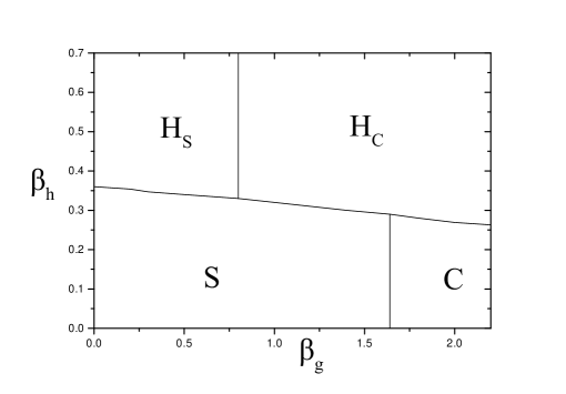
Figure 1: Phase diagram for the isotropic model and for $\beta_{R}=0.01.$ With the help of the hysteresis loops all the phase transition lines turn out to be first order.

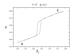
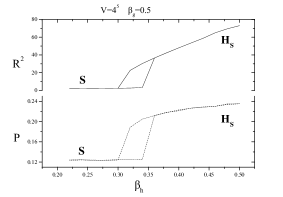
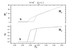
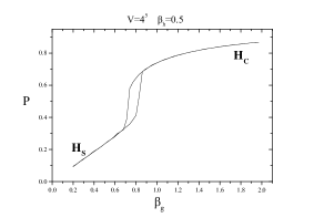
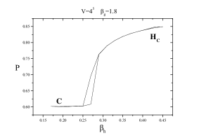
Figure 2: Sample runs on $4^{5}$ lattice volumes. (a) An example for the $S-C$ phase transition where the plaquette is depicted, for $\beta_{h}=0.2$. (b) The $S-H_{S}$ phase transition for $\beta_{g}=0.5$ where the plaquette and $R^{2}$ behaviour are shown. (c) The $S-H_{C}$ phase transition for $\beta_{g}=1.2$ (d) The $H_{S}-H_{C}$ phase transition for $\beta_{h}=0.5$ for the plaquette values showing clearly the transition from the Confining to Coulomb phase of U(1) gauge symmetry. (e) The plaquette hysteresis loop for the $C-H_{C}$ phase transition at $\beta_{g}=1.8$.

In figure 1 we may also see the limiting cases that we described previously and how they form part of the full phase diagram. Within $S$ and $C$ we are in the phase with unbroken symmetry, where $R^{2}\sim 1.$ The phases $H_{S}$ and $H_{C}$ are characterized by a value of $R^{2}$ substantially bigger than $1.$ The phase transitions appear to be first order, since they exhibit large hysteresis loops.

In the sequel (figure 2) we will present some of the results that we used to derive the phase diagram. In figure 2(a) we depict the plaquette as a function of $\beta_{g}$ for $\beta_{h}=0.2.$ This line in the parameter space crosses the $S-C$ phase transition line. One may check that the expression $\displaystyle{\frac{\beta_{g}}{4}}$ slightly underestimates the plaquette (but it is quite close). The deviation is bigger for the Coulomb phase. We should remark here that the analytical expression for the weak coupling systematically overestimates the result.

Figure 2(b) contains results concerning the $S-H_{S}$ phase transition. $\beta_{g}$ is set to 0.5 and $\beta_{h}$ runs. We see the rise of $R^{2}$ as $\beta_{h}$ crosses the phase transition line, signaling the onset of the Higgs phase. A very large hysteresis loop appears, indicating a first order transition. The plaquette value yields some hints about the symmetry group prevailing in each phase. For small values of $\beta_{h}$ the plaquette equals $\displaystyle{\frac{\beta_{g}}{4}}=0.125$ with very good precision, so it corresponds to the strong coupling phase of a pure $SU(2)$ model. For large values of $\beta_{h}$ the remaining symmetry is presumably $U(1).$ This is indeed consistent with the value of the plaquette, which, for large enough $\beta_{h},$ tends to the value $\displaystyle{\frac{\beta_{g}}{2}}=0.250,$ which is the signature of the strong coupling phase of $U(1).$ Consequently, we are in the strong coupling regime of the $U(1)$ which survives the Higgs transition.

Figure 2(c) contains material on the $S-H_{C}$ transition. Here $\beta_{g}$ is set to 1.2. Again we check from the value of $R^{2}$ that we move to a Higgs phase; the phase transition takes place at about $\beta_{h}=0.30.$ Before the transition the plaquette equals $\displaystyle{\frac{\beta_{g}}{4}}=0.30$ to a very good precision, so we start again with the $SU(2)$ strong coupling phase. After the phase transition the plaquette tends to the value $1-\displaystyle{\frac{1}{5\beta_{g}}}=0.83,$ which characterizes the weak coupling phase of five-dimensional $U(1).$

In figure 2(d) we depict the transition from $H_{S}$ to $H_{C}:$ $\beta_{h}$ is set to a large value, $\beta_{h}=0.5,$ to make sure that we are in the Higgs phase, and $\beta_{g}$ runs. The plaquette in $H_{S}$ behaves as $\displaystyle{\frac{\beta_{g}}{2}}$ (strong $U(1)),$ while after the transition it follows the curve $1-\displaystyle{\frac{1}{5\beta_{g}}}.$

Finally, figure 2(e) contains information on the $C-H_{C}$ phase transition: $\beta_{g}$ is set to the large value 1.8 and $\beta_{h}$ varies. We start with the value 0.61 for the plaquette, which is well approximated by the formula $1-\displaystyle{\frac{3}{5\beta_{g}}}.$ Anyway this value characterizes the weak $SU(2).$ After the transition the plaquette tends to the value $1-\displaystyle{\frac{1}{5\beta_{g}}}=0.89,$ that is to a weak $U(1)$ theory.

The hysteresis loops are quite sizeable and they indicate that the phase transitions are of first order.

3.2 The Anisotropic Model

The phase diagram of the anisotropic model is expected to be much richer than the one of the isotropic model, studied in the previous paragraph. The parameter space is very large (consisting of the parameters $\beta_{g},\beta_{g}^{\prime},\beta_{h},\beta^{\prime}_{h},\beta_{R}),$ so a crucial step is to decide which subspace is interesting to investigate. Of course we set $\beta_{R}=0.01$ as before. On the other hand we know the behaviour of the system in the four-dimensional limit. If $\beta_{g}^{\prime}=0$ and $\beta_{h}^{\prime}=0,$ the system becomes strictly four-dimensional. Here also, the qualitative features of the phase diagram are well known since a long time [12]: The four-dimensional model will have a strong-coupling phase $S,$ for relatively small values of $\beta_{h},$ and a four-dimensional Higgs phase, $H_{4},$ for large values of $\beta_{h}.$ The $U(1)$ symmetry which survives in the Higgs phase $H_{4}$ has a phase transition separating a strong from a weak phase. The problem is what will happen when the “primed” quantities $\beta_{g}^{\prime}$ and $\beta_{h}^{\prime}$ take on non-zero values. We will first determine the phase diagram on the $\beta_{g}^{\prime}-\beta_{h}$ plane, for $\beta_{h}^{\prime}=0.001$ at selected values of $\beta_{g}.$ Later on, we will study the role of $\beta_{h}^{\prime}.$

We now choose the values of $\beta_{g}$ for which we will scan the $\beta_{g}^{\prime}-\beta_{h}$ plane. The first value will be $\beta_{g}=0.5,$ since we would like to have a value of $\beta_{g}$ lying in the strong coupling regime. Note that (referring to figure 1), in the isotropic model, if one starts at $\beta_{g}=0.5,$ for large enough $\beta_{h}$ one will end up into the strong coupling Higgs phase, $H_{S}.$ An interesting remark is that the confinement scale, which is contained naturally in the theory at $\beta_{g}=0.5,$ may serve as a cut-off; the cut-off is necessary to define a non-renormalizable model, such as this one. For completeness we also choose the value $\beta_{g}=1.2,$ for our second set of measurements. The difference from the $\beta_{g}=0.5$ case is that, in the isotropic model, one ends up with the weakly coupled Higgs phase $(H_{C}),$ if $\beta_{h}$ is set to a large value. We do not try any value of $\beta_{g},$ which corresponds to the five-dimensional Coulomb phase of $SU(2),$ that is $\beta_{g}>1.63,$ since starting from a weakly coupled $SU(2)$ it is unlikely that one may end up with a layered phase, which is the main subject of the present work. Thus we will only study the values $\beta_{g}=0.5$ and $\beta_{g}=1.2.$

It is interesting to point out that the criterion that we used in the previous paragraph to discriminate between phases, namely the behaviour of the plaquettes for strong and weak couplings needs to be modified. This is necessary, since, for instance, $\beta_{g}$ may lie in the weak coupling range, while $\beta_{g}^{\prime}$ may be strong. In addition we may encounter space-times with effective dimensions 4 or 5, so the expressions concerning the weak coupling will also change. A first guess at the behaviour of the plaquettes is that $P_{S}$ will behave as $\displaystyle{\frac{\beta_{g}}{4}}$ in the strong $SU(2)$ regime and as $1-\displaystyle{\frac{3}{D\beta_{g}}}$ in the weak coupling $SU(2)$ for D dimensions. Correspondingly, $P_{T}$ will be given by similar expressions, with $\beta_{g}$ replaced by $\beta_{g}^{\prime}.$ The behaviours of the plaquettes if the surviving symmetry is $U(1)$ read $\displaystyle{\frac{\beta_{g}}{2}},\ 1-\displaystyle{\frac{1}{D\beta_{g}}}$ for $P_{S}$ and $\displaystyle{\frac{\beta^{\prime}_{g}}{2}},\ 1-\displaystyle{\frac{1}{D\beta_{g}^{\prime}}}$ for $P_{T}.$ It turns out that these expressions are not very good approximations. They give the qualitative flavour of each phase but are less accurate than the corresponding formulae of the isotropic model. We now proceed with the study of the two chosen values of $\beta_{g}.$

$\bullet$   $\mathbf{\beta_{g}=0.5}$

We begin by giving the phase diagram that we obtain, as we did with the isotropic model. Later on we will give the results of some of the runs that we used to derive the phase diagram. The phase diagram is depicted in figure 3 and has three phases: The Strong, confining phase $S,$ the “layered”, four-dimensional Higgs phase, $H_{4},$ and the five-dimensional Higgs phase, $H_{5}.$ Let us explain briefly what we understand about these phases. The $S$ and $H_{5}$ phases are fairly easy to understand: they are the five-dimensional phases with unbroken and broken symmetry respectively. The expected behaviours of the plaquettes are given in table 1. In particular, in the confining phase $S,$ $P_{S}$ and $P_{T}$ will behave as $\displaystyle{\frac{\beta_{g}}{4}}$ and $\displaystyle{\frac{\beta^{\prime}_{g}}{4}}$ respectively. In the $H_{5}$ phase the $SU(2)$ symmetry will be broken down to a (weak coupling) $U(1),$ so the behaviours of $P_{S}$ and $P_{T}$ are $1-\displaystyle{\frac{1}{5\beta_{g}}}$ and $1-\displaystyle{\frac{1}{5\beta^{\prime}_{g}}}$ respectively. The $H_{4}$ phase needs some clarifications. When $\beta_{g}^{\prime}=0,\beta_{h}^{\prime}=0,$ we expect that the system will be strictly four-dimensional. When $\beta_{g}^{\prime}$ and $\beta_{h}^{\prime}$ are small (but non-zero), we expect that we may have some kind of layer structure (that is, almost four-dimensional), which is characterized by small transverse-like quantities and large space-like ones. This is the phase that we have denoted by $H_{4}.$ However, in this case, it is not only the transverse direction which is confining $\left(P_{T}\sim\displaystyle{\frac{\beta^{\prime}_{g}}{4}}\right),$ but also the space-like behaviour is dominated by the strong coupling $\beta_{g}=0.5,$ that is $P_{S}\sim\displaystyle{\frac{\beta_{g}}{2}}.$ In other words, we have a strong coupling confining behaviour both in the transverse direction (where the $SU(2)$ symmetry remains intact, and the denominator is $4)$ and within the layer, where the symmetry is broken down to $U(1),$ which is the reason behind the denominator $2.$ Thus in this phase we have $SU(2)$ confinement along the extra fifth direction, and $U(1)$ confinement within the layers. Since by the term layered phase we mean a situation with confinement in the transverse direction and Coulomb behaviour within the layers, we remark here that this term is not proper here, so we should enclose the word layered in quotes in this case. Let us note that the two Higgs phases are characterised primarily by large values for the space–like link $L_{S}$ and the measure squared $R^{2}$. An important remark is that within $H_{4}$ the $SU(2)$ symmetry does not break down to $U(1)$ in the transverse direction. It is only within the layers that the symmetry group changes.

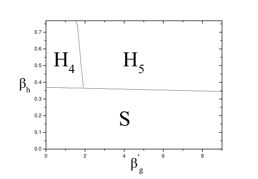
Figure 3: Phase diagram for the anisotropic model for $\beta_{g}=0.5$ and $\beta_{R}=0.01.$ Using the hysteresis loops all the phase transition lines turn out to be first order.

	Layer	Transverse direction
S	SU(2)–strong: $P_{S}\sim\displaystyle{\frac{\beta_{g}}{4}}$	SU(2)–strong: $P_{T}\sim\displaystyle{\frac{\beta^{\prime}_{g}}{4}}$
$\mathbf{H_{4}}$	U(1)–strong: $P_{S}\sim\displaystyle{\frac{\beta_{g}}{2}}$	SU(2)–strong: $P_{T}\sim\displaystyle{\frac{\beta^{\prime}_{g}}{4}}$
$\mathbf{H_{5}}$	U(1)–5D Coulomb: $P_{S}\sim 1-\displaystyle{\frac{1}{5\beta_{g}}}$	U(1)–5D Coulomb: $P_{T}\sim 1-\displaystyle{\frac{1}{5\beta^{\prime}_{g}}}$

Table 1: Phase characterization in terms of $P_{S}$ and $P_{T}$ values for $\beta_{g}=0.5$.

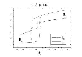
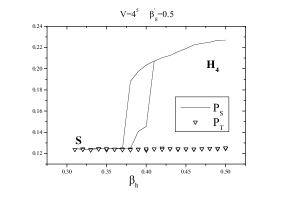
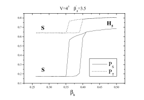
Figure 4: Examples concerning the anisotropic model for $\beta_{g}=0.5$. (a) The $H_{4}-H_{5}$ phase transition. (b) The $S-H_{4}$ phase transition. (c) The $S-H_{5}$ phase transition.

Let us examine in some more detail the behaviour of the various quantities across the phase transitions.

In figure 4(a) we have set $\beta_{h}=0.42,$ so that the system is in the Higgs phase, and we let $\beta_{g}^{\prime}$ run. Considering $P_{T}$ we see that it initially equals $\displaystyle{\frac{\beta_{g}^{\prime}}{4}},$ which signals $SU(2)$ confinement, while after the transition it tends asymptotically to the value $1-\displaystyle{\frac{1}{5\beta_{g}^{\prime}}},$ that is to a Coulomb phase of $U(1).$ Thus we observe the breaking of the symmetry group in the transverse direction. On the other side of the transition $P_{S}$ starts with a value quite close to $\displaystyle{\frac{\beta_{g}}{2}}=0.250,$ while after the phase transition it approaches asymptotically the value $1-\displaystyle{\frac{1}{5\beta_{g}}}=0.60.$ Thus within the layers we have a transition from $U(1)$ confinement to a $U(1)$ Coulomb phase. The above findings are consistent with a transition from $H_{4}$ to $H_{5}.$

The changes across the $S-H_{4}$ transition are shown in figure 4(b). $\beta_{g}^{\prime}$ has been set to 0.5 (equal to $\beta_{g})$ and the $\beta_{h}$ coupling runs. It turns out that $P_{T}$ is equal to $\displaystyle{\frac{\beta_{g}^{\prime}}{4}}=0.125$ in both phases. On the contrary, $P_{S}$ equals $\displaystyle{\frac{\beta_{g}}{4}}=0.125$ (equal to $P_{T})$ in the strong coupling phase, while after the transition it approaches (for large enough $\beta_{h})$ the value $\displaystyle{\frac{\beta_{g}}{2}}=0.250,$ which characterizes the $U(1)$ symmetry. Thus the system moves from $S$ to $H_{4}.$ An intriguing feature is that the value $\beta_{g}=0.5$ is considered as strong coupling in the $S$ phase and the $H_{4}$ phase (this paragraph) and as weak coupling in the $H_{5}$ phase (figure 4(a)). This means that it is not just the value of a specific coupling that counts, but also the values of the remaining couplings; in particular the decisive element is the phase in which the system lies.

Finally figure 4(c) contains data for $\beta^{\prime}_{g}=3.5$ and running $\beta_{h}.$ The space-like plaquette has the value $\displaystyle{\frac{\beta_{g}}{4}}=0.125$ for small $\beta_{h},$ so it exhibits $SU(2)$ confinement, consistent with an $SU(2)$ strong $(S)$ phase. For large $\beta_{h}$ it tends to values consistent with $1-\displaystyle{\frac{1}{5\beta_{g}}}=0.60.$ On the other hand $P_{T}$ starts from strong coupling values about 0.64. We again remark that the apparently weak coupling $\beta_{g}^{\prime}=3.5$ yields strong coupling behaviour, since the system is in an appropriate phase, due to the values of the remaining couplings. For large $\beta_{h},$ $P_{T}$ tends to the limit $1-\displaystyle{\frac{1}{5\beta_{g}^{\prime}}}=0.94$ and it appears safe to conclude that the system moves from $S$ to $H_{5}.$ The essential difference between the two $S-H$ transitions lies in the fact that $P_{T}$ does not change at all during the $S-H_{4}$ transition, but changes from strong $SU(2)$ to weak $U(1)$ during the $S-H_{5}$ transition. The link $L_{T}$ follows the same scheme.

Thus we have explained how the phase diagram has been derived. We should note the absence of a $SU(2)$ Coulomb phase for large values of $\beta_{g}^{\prime}.$ It has not been possible to find it, although we have searched for it up to $\beta_{g}^{\prime}\sim 10$. This result may be attributed to the small chosen value of $\beta_{g}.$ The argument goes as follows: let us fix the gauge by requiring that $U_{5}(x)=1.$ Then the transverse-like plaquettes are in principle driven by $\beta_{g}^{\prime}.$ If $\beta_{g}$ is large enough, it will couple the neighbouring transverse-like hyperplanes, e.g. the $\hat{5}\hat{1}$ and $\hat{5}\hat{2}.$ However, if $\beta_{g}$ is small (which is the case here) these hyperplanes will decouple and the model will reduce to several copies of the same two-dimensional $SU(2)$ gauge model, which does not exhibit phase transitions.

$\bullet$   $\mathbf{\beta_{g}=1.2}$

As we already stated, we also simulated the system at a larger value of $\beta_{g},$ namely $1.2,$ to study its behaviour at weaker couplings. Two striking new features arise: an $SU(2)$ Coulomb phase and a genuine layered $(H_{4})$ phase with Coulomb (rather than strong) $U(1)$ interations within the layer. As in the previous paragraph, we give the resulting phase diagram in figure 5 and summarize the behaviours of the plaquettes in the various phases in table 2. Next we will elaborate on the phase transition lines in more detail and explain how our claims in figure 5 and table 2 are derived.

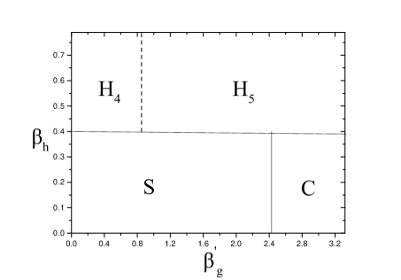
Figure 5: Phase diagram for the anisotropic model for $\beta_{g}=1.2$ and for $\beta_{R}=0.01.$

	Layer	Transverse direction
S	SU(2)–strong: $P_{S}\sim\displaystyle{\frac{\beta_{g}}{4}}$	SU(2)–strong: $P_{T}\sim\displaystyle{\frac{\beta^{\prime}_{g}}{4}}$
C	SU(2)–Coulomb: $P_{S}\sim 1-\displaystyle{\frac{3}{5\beta_{g}}}$	SU(2)–Coulomb: $P_{T}\sim 1-\displaystyle{\frac{3}{5\beta^{\prime}_{g}}}$
$\mathbf{H_{4}}$	U(1)–4D Coulomb: $P_{S}\sim 1-\displaystyle{\frac{1}{4\beta_{g}}}$	SU(2)–strong: $P_{T}\sim\displaystyle{\frac{\beta^{\prime}_{g}}{4}}$
$\mathbf{H_{5}}$	U(1)–5D Coulomb: $P_{S}\sim 1-\displaystyle{\frac{1}{5\beta_{g}}}$	U(1)–5D Coulomb: $P_{T}\sim 1-\displaystyle{\frac{1}{5\beta^{\prime}_{g}}}$

Table 2: Table 2: Phase characterization in terms of the $P_{S}$ and $P_{T}$ values for $\beta_{g}=1.2$.

A new phase transition line is the one separating the strong $S$ phase from the Coulomb $C$ phase. An example of the transition is given in figure 6(a), where $\beta_{h}=0.01$ and $\beta_{g}^{\prime}$ runs. In the strong phase $S$ both $P_{S}$ and $P_{T}$ take a value equal to the $\displaystyle{\frac{1}{4}}$ of their respective lattice couplings, while their values get large when the system is passes over to the Coulomb phase $C.$ In particular, $P_{S}$ tends to the value $1-\displaystyle{\frac{3}{5\beta_{g}}}=0.5,$ while $P_{T}$ follows the curve $1-\displaystyle{\frac{3}{5\beta_{g}^{\prime}}}.$ The $S-C$ phase transition appears to be first order since there is a clear hysteresis loop for the relevant points although not a very large one.

In figure 6(b) we show $P_{S},P_{T}$ and $L_{T}$ as the system moves from $H_{4}$ to $H_{5}.$ There is no significant hysteresis loop in any of the three quantities, so the transition is presumably a continuous phase transition or a crossover. The transverse-like link $L_{T}$ moves from a small value in $H_{4}$ to a large value in $H_{5},$ which is actually what one would expect. One can make more quantitative remarks about the two plaquettes. The space-like plaquette $P_{S}$ does not really feel the phase transition very much. The only aspect that changes, from the point of view of $P_{S},$ is that the four-dimensional space-time becomes five-dimensional. On the basis of what has been already mentioned, in $H_{4}$ the space–like plaquette, $P_{S}$, should approach the value $1-\displaystyle{\frac{1}{4\beta_{g}}}=0.79,$ while in $H_{5}$ the value $1-\displaystyle{\frac{1}{5\beta_{g}}}=0.83.$ Thus one would expect a slight increase in the value of $P_{S}$ during the phase transition which is actually observed. On the other hand, the transverse-like plaquette $P_{T}$ starts with the strong coupling value $\displaystyle{\frac{\beta_{g}^{\prime}}{4}},$ which is expected for the confining $SU(2),$ and ends up with $1-\displaystyle{\frac{1}{5\beta_{g}^{\prime}}},$ which characterizes the five-dimensional Coulomb $U(1)$ associated with the $H_{5}$ phase.

As we already said, a very important point is the emergence of a genuine layered phase. The transition $S-H_{4}$ is shown in figure 6(c) and illuminates some properties of $H_{4}.$ To begin with, $R^{2}$ starts from a small value and ends up with values much larger than 1. This ensures that the system moves into a Higgs phase. The space-like plaquette $P_{S}$ starts with the strong coupling value $\displaystyle{\frac{\beta_{g}}{4}}=0.30$ and tends after the transition to the four-dimensional Coulomb $U(1)$ value $1-\displaystyle{\frac{1}{4\beta_{g}}}=0.79.$ This is in sharp contrast with the behaviour of $P_{S}$ in $H_{4}$ in the $\beta_{g}=0.5$ case, figure 4(b), where it followed $\displaystyle{\frac{\beta_{g}}{2}},$ implying strong $U(1).$ Here we observe Coulomb behaviour within the layers. In addition, we have used the value $D=4$ for the dimension of space-time to get the value 0.79. If we had used the value $D=5,$ the resulting value would be 0.83. Our results are not conclusive in this respect. The Monte Carlo value is smaller than the analytical prediction anyway. However comparison with figure 6(b) shows that $P_{S}$ is relatively small, since in the $H_{5}$ phase its value would approach 0.8. Thus, it seems that the choice D=4 is correct.

On the other hand one may be confident that the layers are essentially four-dimensional entities, since the values of the transverse-like observables are very small and suggest that the layers are decoupled. In particular $P_{T},$ shown in the same figure, takes the value $\displaystyle{\frac{\beta^{\prime}_{g}}{4}},$ signaling $SU(2)$ confinement in the transverse direction. Thus we have a layered phase, where particles and gauge fields interact through Coulomb $U(1)$ interactions within the four-dimensional layers and cannot escape towards the transverse direction because of the $SU(2)$ confinement forces which prevail in the space between the layers. In figure 6(d) we show the space-like $(L_{S})$ and timelike $(L_{T})$ links respectively. It is clear that $L_{T}$ has a small value throughout, while $L_{S}$ grows. This is because the real phase change takes place within the layer, where the strong $SU(2)$ transforms to four-dimensional $U(1)$ and space-like quantities, such as $L_{S},$ are sensitive to this transition. The existence of the large hysteresis loops suggests a first order phase transition.

Some sample results concerning the transition $S-H_{5}$ are contained in figures 7(a) and 7(b). In figure 7(a) the quantity $R^{2}$ shows that the system moves to a Higgs phase. The space-like plaquette starts with $SU(2)$ confinement behaviour and ends up with Coulomb $U(1)$ behaviour. Similarly, $P_{T}$ starts with $SU(2)$ confinement behaviour and ends up with Coulomb $U(1)$ behaviour. This is consistent with an $S-H_{5}$ transition. The analytical predictions here are not precise at all in this case. In particular, the predictions for the plaquettes in the $H_{5}$ phase are $P_{S}\approx 1-\displaystyle{\frac{1}{5\beta_{g}}}=0.83$ and $P_{T}\approx 1-\displaystyle{\frac{1}{5\beta_{g}^{\prime}}}=0.87.$ However the Monte Carlo results show that $P_{S}>P_{T}.$ Also the analytical result $\displaystyle{\frac{\beta_{g}^{\prime}}{4}}=0.375$ in the phase $S$ does not agree well with the Monte Carlo result 0.48. Thus in this case one should be content with the qualitative features characterizing the phase transition. The link variables of figure 7(b) are also consistent with an $S-H_{5}$ transition. It is remarkable that although we insist on the rather small value $\beta_{h}^{\prime}=0.001,$ the system passes over to the $H_{5}$ phase which is characterised by large values for all order parameters. In addition, the large hysteresis loops suggest a first order transition.

Finally the $C-H_{5}$ transition, which is shown in figure 7(c) also appears to be first order. However the hysteresis loop is small, so more detailed analysis is needed in this case.

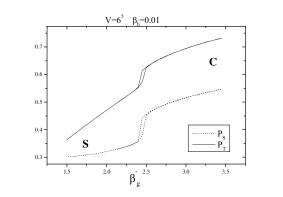
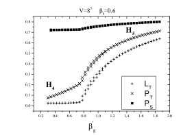
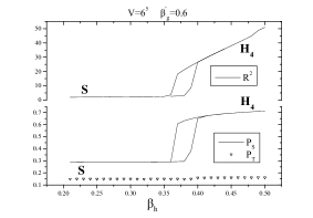
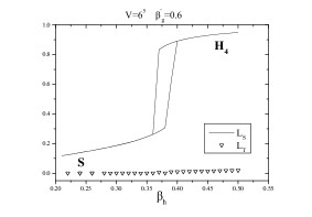
Figure 6: (a) $P_{S}$ and $P_{T}$ for the $S-C$ phase transition. (b) $L_{T}$, $P_{S}$ and $P_{T}$ for the $H_{4}-H_{5}$ phase transition. (c) $R^{2},P_{S}$ and $P_{T}$ for the $S-H_{4}$ phase transition. (d) $L_{S}$ and $L_{T}$ for the $S-H_{4}$ phase transition.

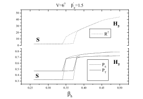
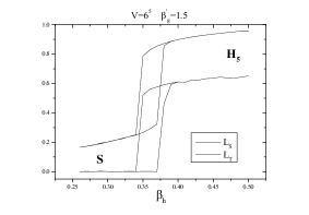
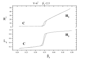
Figure 7: (a) $R^{2},P_{S}$ and $P_{T}$ for the $S-H_{5}$ phase transition. (b) $L_{S}$ and $L_{T}$ for the $S-H_{5}$ phase transition. (c) $R^{2}$ and $L_{S}$ for the $C-H_{5}$ phase transition.

3.3 The effect of $\beta_{h}^{\prime}$

In this paragraph we go ahead with some results concerning the effects of the $\beta_{h}^{\prime}$ coupling, which has been set to the value 0.001 up to now. In figure 8 we have fixed the couplings to the values $\beta_{g}=1.2,\ \beta_{h}=0.45,\ \beta_{R}=0.01$ and performed a scanning in $\beta_{h}^{\prime}$ at two values of $\beta_{g}^{\prime}.$ The order parameter considered is the transverse-like plaquette $P_{T}.$ For $\beta_{g}^{\prime}=0.4$ we see that we start from an $SU(2)$ confining theory for small $\beta_{h}^{\prime}$ (the value of the plaquette equals $\displaystyle{\frac{\beta_{g}^{\prime}}{4}}=0.1)$ to end up with a $U(1)$ confining theory, since the value of $P_{T}$ tends to $\displaystyle{\frac{\beta_{g}^{\prime}}{2}}=0.2.$ The space–like plaquette $P_{S}$ takes on big values and it seems to indicate that the layers remain in the Coulomb phase. One may be tempted to think that it is a layered phase. However, a look at figure 9, which contains the corresponding links, reveals something strange: for large enough $\beta_{h}^{\prime}$ the transverse-like link is not small, as one would expect from a layered phase. The physical understanding of this situation is that the gauge field cannot really travel from a layer to the neighbouring one. However, since we have arranged the couplings to place the system in the Higgs phase, symmetry breaking has occured, resulting in a $U(1)$ residual symmetry along with a scalar particle with zero charge. Nothing can prevent this particle from moving over the whole lattice, which has the result of giving a large value for $L_{T},$ as we see in figure 9. We remark that $L_{T}$ is the gauge invariant propagator of the scalar particle at the distance of one lattice spacing. This physical situation has not been encountered before. It is a new phase, which contains $U(1)$ gauge fields localized within the layers and a freely moving scalar field. One may like to call this phase $C_{4},$ since the scalar field does not play any significant role. It is a gauge field in a four-dimensional Coulomb phase coupled to a massive scalar.

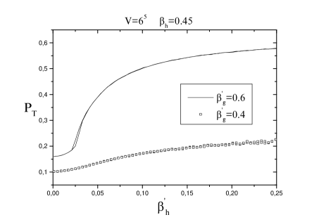
Figure 8: The transverse-like plaquette at $\beta_{g}=1.2,\beta_{h}=0.45$ and $\beta_{R}=0.01$ for $\beta_{g}^{\prime}=0.4$ and $\beta_{g}^{\prime}=0.6.$

At $\beta_{g}^{\prime}=0.6$ we have the upper curve of figure 8. The system starts at the $SU(2)$ confining phase with $P_{T}$ taking the value $\displaystyle{\frac{\beta_{g}^{\prime}}{4}}=0.15,$ but the final phase appears to be weakly coupled $U(1),$ with $P_{T}\approx 1-\displaystyle{\frac{1}{5\beta_{g}^{\prime}}}=0.67.$ The transverse-like link is also large in this case for the same reason. If one would like to give a name to this phase, one would call it $C_{5}.$ We observe that, although at $\beta_{g}^{\prime}=0.4$ there is no trace of a phase transition between strong $SU(2)$ and strong $U(1),$ the transition from strong $SU(2)$ to weak $U(1)$ at $\beta_{g}^{\prime}=0.6$ exhibits a (small) hysteresis loop in between, signaling a possible phase change. We remark here that the value $\beta_{h}^{\prime}=0.001$ that we used for most of our Monte Carlo simulations is rather small; in particular it lies before the phase transition for $\beta_{g}^{\prime}=0.6$ of figure 8.

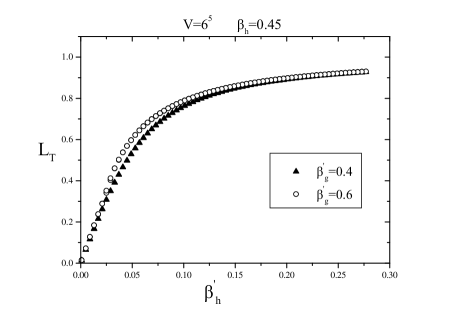
Figure 9: The transverse-like link at $\beta_{g}=1.2,\beta_{h}=0.45$ and $\beta_{R}=0.01$ for $\beta_{g}^{\prime}=0.4$ and $\beta_{g}^{\prime}=0.6.$

A remark concerning figure 9 is that the curve for for $\beta_{g}^{\prime}=0.6$ is steeper than the one for $\beta_{g}^{\prime}=0.4.$ Thus we expect (actually verified) that for bigger values of $\beta_{g}^{\prime}$ it will be even steeper, meaning that if $\beta_{g}^{\prime}$ is large enough, even a small value of $\beta_{h}^{\prime}$ is enough to take the system out of the $SU(2)$ confinement.

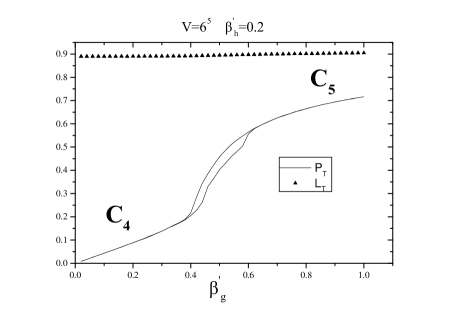
Figure 10: The transverse-like plaquette and link at $\beta_{g}=1.2,\beta_{h}=0.45$ and $\beta_{R}=0.01$ for $\beta_{h}^{\prime}=0.2$ and running $\beta_{g}^{\prime}.$

From figure 8 we see that if we set $\beta_{h}^{\prime}=0.20$ and let $\beta_{g}^{\prime}$ run, we should see a change in the behaviour of the system between $\beta_{g}^{\prime}=0.4$ and $\beta_{g}^{\prime}=0.6.$ The results of this run is displayed in figure 10. The transverse-like link takes a large value, the same in both the $C_{4}$ and $C_{5}$ phases, while $P_{T}$ follows $\displaystyle{\frac{\beta_{g}^{\prime}}{2}}$ in the beginning and then changes to $1-\displaystyle{\frac{1}{5\beta_{g}^{\prime}}},$ with a hysteresis loop in between.

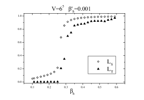
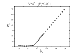
Figure 11: Graphs derived by hysteresis loop technique for the pure scalar field showing the $L_{S}$, $L_{T}$ (fig.(a)) and $R^{2}$ (fig. (b)) as $\beta^{\prime}_{h}=0.001$ and $\beta_{h}$ is running.

3.4 The role of the scalar field

We would like to study the role of the scalar field in the formation of the layered phase, so we simulate our model setting the lattice gauge couplings $\beta_{g}$ and $\beta_{g}^{\prime}$ to infinity. Thus the gauge fields do not play role any more and we are left with the dynamics of the scalar fields. In a sense figure 11, which we will present shortly, is similar to figure 7(c), with the difference that $\beta_{g}$ and $\beta_{g}^{\prime}$ are infinite rather than taking a finite value. The results on the hysteresis loops for $L_{S}$ and $L_{T}$ of the pure scalar field model are shown in figure 11. We have set $\beta_{h}^{\prime}=0.001,$ while $\beta_{h}$ is running. One can see that there is a possible phase transition near $\beta_{h}=0.25$ (which is a reasonable critical point, since one would expect the value $\displaystyle{\frac{1}{D-1}},$ with $D=5$). Before the phase transition we have a symmetric phase (since $R^{2}$ is small, as shown in figure 11(b)); in addition $L_{T}$ is zero in this phase, so we conclude that the system actually consists of four-dimensional layers. After the transition $R^{2}$ becomes large and the two links take large, almost equal values. Thus, the system moves presumably towards a five-dimensional Higgs phase, $H_{5}.$

An interesting issue is the dependence of $L_{T}$ on the value of $\beta_{h}^{\prime}.$ In figure 11(a) (that is, for $\beta_{h}^{\prime}=0.001)$ the transverse-like link $L_{T}$ takes a large value if $\beta_{h}$ becomes large enough. Thus it appears that no $H_{4}$ phase appears. On the other hand we know that if $\beta_{h}^{\prime}=0$ the scalar model is strictly four-dimensional. Thus we expect some phase transition between the two values $\beta_{h}^{\prime}=0$ and $\beta_{h}^{\prime}=0.001.$ The question is whether the phase transition takes place exactly at $\beta_{h}^{\prime}=0$ or at some small but non-zero value. To this end we have measured $L_{T}$ for small values of $\beta_{h}^{\prime}$ and present the results in table 3. For each value of $\beta_{h}^{\prime}$ we present the statistical average of $L_{T}$ in the second column along with the limits within which this quantity fluctuates in columns three and four. One may easily see that for $\beta_{h}^{\prime}$ smaller than about $10^{-5}$ the transverse-like link $L_{T}$ is compatible with zero, while the fluctuations are large. The mean value $L_{T}$ increases with $\beta_{h}^{\prime}$, while the fluctuation range decreases.

It appears that $L_{T}$ is zero for small $\beta_{h}^{\prime}.$ It seems that there exists a critical value for $\beta_{h}^{\prime}$ above which $L_{T}$ takes on a non-zero value. However, it is possible that the existence of a non-zero critical value might be a volume effect. In particular this critical value (which lies between $10^{-5}$ and $10^{-4}$ for the $6^{5}$ volume considered in table 4) may tend to zero as the volume is increased. In other words it is possible to have this phase change exactly at $\beta_{h}^{\prime}=0.$ To investigate this issue we have set $\beta_{h}^{\prime}$ to two small values, namely $10^{-4}$ and $10^{-5}$ and measured $L_{T}$ for various volumes. For $\beta_{h}^{\prime}=10^{-4}$ we see in table 4 that we have wild fluctuations and a small mean value for the $4^{5}$ volume, while for bigger volumes the fluctuations are drastically reduced and the average increases accordingly. Thus, if one would stop at $4^{5},$ one might think that the coupling $\beta_{h}^{\prime}=10^{-4}$ lies in the region where $L_{T}=0.$ However, we see readily that this depends very much on the volume used: for larger volumes the same coupling lies in the regime where $L_{T}\neq 0.$ One may try to move to even smaller values for $\beta_{h}^{\prime},$ for example the value $10^{-5}$ shown on the right part of table 4. This value appears to be in the $L_{T}=0$ region for both $4^{5}$ (not shown) and $6^{5}$ lattices. However, if we move to the $8^{5}$ volume, it also gives non-zero values for $L_{T}.$ It seems safe to conclude that the critical value of $\beta_{h}^{\prime}$ for infinite volume is actually $\beta_{h}^{\prime}=0.$ Perhaps one should also explore smaller values of $\beta_{h}^{\prime}$ to corroborate this conclusion, however we claim that, since we have checked down to values of the order of $\displaystyle{\frac{1}{V}},$ this conclusion holds true.

$\beta_{h}^{\prime}$	$L_{T}$	$L_{low}$	$L_{high}$
$0.00$	-0.059	-0.65	0.46
$10^{-7}$	-0.075	-0.69	0.44
$10^{-5}$	0.015	-0.60	0.75
$10^{-4}$	0.745	0.41	0.93
$10^{-3}$	0.948	0.89	0.98
$10^{-2}$	0.968	0.91	0.99

Table 3: Behaviour of $L_{T}$ and the limits of its statistical fluctuations for the pure scalar field for a $6^{5}$ lattice.

$\beta_{h}^{\prime}=10^{-4}$				$\beta_{h}^{\prime}=10^{-5}$
V	$L_{T}$	$L_{low}$	$L_{high}$	V	$L_{T}$	$L_{low}$	$L_{high}$
$4^{5}$	0.258	-0.54	0.94	$6^{5}$	0.15	-0.60	0.75
$6^{5}$	0.745	0.41	0.93	$8^{5}$	0.890	0.80	0.95
$8^{5}$	0.934	0.87	0.96	$10^{5}$	0.915	0.83	0.97

Table 4: Behaviour of $L_{T}$ and the limits of its statistical fluctuations for the pure scalar field. Two values for $\beta_{h}^{\prime}$ are explored for various lattice volumes.

In conclusion, we have not found any sign of four-dimensional (layered) Higgs phase for the scalar model. Its absence can be attributed to the lack of gauge interactions which could provide the mechanism for confinement along the transverse direction. This leads to the conclusion that if one wants to have a layered phase in realistic theories with localization of the fields within a four–dimensional subspace (in the framework of a theory in higher dimensions), gauge field interactions are necessary. Similar conclusions have been reached by Fu and Nielsen [18] through a mean field treatment of the $O(N)$ model. The “localization scale” (i.e. the energy above from which the extra dimension becomes visible) appears to be determined by the gauge coupling constants. On the other hand, we have already mentioned that a pure $SU(2)$ gauge theory has no layer phase in five dimensions. It appears that a coordinated action of the gauge and scalar sectors is necessary to produce a layered phase in 5 dimensions, since each sector on its own cannot be efficient in this respect.

4 Concluding Remarks

In this paper we have tried to find a layer phase in the SU(2)–adjoint Higgs model in five dimensions using lattice simulations. Apart from exploring the phase diagram for the isotropic model we focused our attention to the anisotropic one. We determined the phase diagram in the $\beta_{h}-\beta_{g}^{\prime}$ hyperplane of the lattice parameter space and we found out that there is a four–dimensional layered Higgs phase exhibited by the model which is separated by a phase boundary from the strong phase. This is an entirely new result which is attributed to the gauge–scalar interaction considered. Let us recall the well-known result that the pure SU(2) gauge theory exhibits a layered structure in six dimensions only and yields a non-physical Coulomb layered phase in five dimensions. The other new and interesting feature of the model is that for some region of the lattice couplings the formation of the layered Higgs phase is attributed to the SU(2) strong interaction along the transverse–extra dimension. This fact serves as an important physical indication of the way that four dimensional layers may be formed.
The whole construction may have interesting implications on models based on grand unified groups, such as $SU(5),$ with the scalars in the adjoint representation (for example the one with dimension 24) defined in a higher–dimensional space. From this model we could get a layered phase in four dimensions. The model would be promising if the relevant scale of this layer formation would be of the same order of magnitude as the scale of the symmetry breaking from SU(5) down to $\mbox{SU(3)}\times\mbox{SU(2)}\times\mbox{U(1)}$.

Acknowledgements

The authors acknowledge partial financial support by the TMR Network entitled “Finite Temperature phase transitions in Particle Physics”, EU contract number FMRX-CT97-0122. K.F. thanks C. Bachas and C. Korthals–Altes for useful discussions.

Appendix: Mean Field Analysis

Our starting point is the partition function

$$Z=\prod_{x}\int\prod_{\mu=1}^{5}dU_{\mu}(x)\int d\Phi(x)e^{-S(a_{\mu}^{M},e^{m})},\quad S(a_{\mu}^{M},e^{m})=S_{G}+S_{GH}+S_{H},$$ (7)

where

$$S_{G}=-\frac{\beta_{g}}{2}\sum_{x,\mu<\nu<5}Tr[U_{\mu}(x)U_{\nu}(x+\hat{\mu})U^{\dagger}_{\mu}(x+\hat{\nu})]U^{\dagger}_{\nu}(x)-\frac{\beta_{g}^{\prime}}{2}\sum_{x,\mu<5}Tr[U_{\mu}(x)U_{5}(x+\hat{\mu})U^{\dagger}_{\mu}(x+\hat{5})U^{\dagger}_{5}(x)],$$

$$S_{GH}=-\frac{\beta_{h}}{2}\sum_{x,\mu<5}Tr[\Phi(x)U_{\mu}(x)\Phi(x+\hat{\mu})U^{\dagger}_{\mu}(x)]-\frac{\beta_{h}^{\prime}}{2}\sum_{x}Tr[\Phi(x)U_{5}(x)\Phi(x+\hat{5})U^{\dagger}_{5}(x)],$$

$$S_{H}=\beta_{R}\sum_{x}\left(\frac{1}{2}Tr\Phi^{2}-1\right)^{2}.$$

We note in addition that

$$\Phi(x)=\phi^{m}(x)\sigma^{m},\phi^{m}(x)\equiv\rho(x)e^{m}(x)=\rho(x)(\sin\theta(x)\cos\psi(x),\sin\theta(x)\sin\psi(x),\cos\theta(x))$$

and

$$d\Phi(x)=\frac{1}{\pi^{3/2}}e^{-\rho^{2}(x)}\rho^{2}(x)d\rho(x)d\cos\theta(x)d\psi(x)\equiv e^{-\rho^{2}(x)}\rho^{2}(x)d\rho(x)de(x),$$

along with

$$U_{\mu}(x)=a^{0}_{\mu}(x)+i\sum_{m=1}^{3}a_{\mu}^{m}(x)\sigma^{m},$$

$$dU_{\mu}(x)=\frac{1}{\pi^{2}}\delta[(a^{0}_{\mu}(x))^{2}+\sum_{m=1}^{3}(a_{\mu}^{m}(x))^{2}-1]\prod_{M=0}^{3}da_{\mu}^{M}(x).$$

We introduce the unconstrained variables $A_{\mu}^{M}(x),M=0,1,2,3,$ corresponding to the gauge field variables $a_{\mu}^{M}(x),M=0,1,2,3,$ and use the identity:

$$1=\prod_{x}\prod_{M=0}^{3}\prod_{\mu=1}^{5}\int_{-\infty}^{+\infty}dA_{\mu}^{M}(x)\delta(A^{M}_{\mu}(x)-a^{M}_{\mu}(x))=$$

$$=\prod_{x}\prod_{M=0}^{3}\prod_{\mu=1}^{5}\int_{-\infty}^{+\infty}dA_{\mu}^{M}(x)\int_{-i\infty}^{+i\infty}\frac{d\alpha^{M}_{\mu}(x)}{2\pi i}\exp[-\alpha^{M}_{\mu}(x)(A^{M}_{\mu}(x)-a^{M}_{\mu}(x))],$$

We follow a similar path with the unconstrained variables $E^{m}(x),m=1,2,3,$ corresponding to the scalar field variables $e^{m}(x),m=1,2,3,$ which satisfy the identity:

$$1=\prod_{x}\prod_{m=1}^{3}\int_{-\infty}^{+\infty}dE^{m}(x)\delta(E^{m}(x)-e^{m}(x))=$$

$$=\prod_{x}\prod_{m=1}^{3}\int_{-\infty}^{+\infty}dE^{m}(x)\int_{-i\infty}^{+i\infty}\frac{d\epsilon^{m}(x)}{2\pi i}\exp[-\epsilon^{m}(x)(E^{m}(x)-e^{m}(x))].$$

Next we insert the above factors of 1 in the partition function (7) and rearrange the order of the integrations:

$$Z=\int_{-\infty}^{+\infty}\prod_{M=0}^{3}\prod_{\mu=1}^{5}dA_{\mu}^{M}(x)\int_{-i\infty}^{+i\infty}\frac{d\alpha^{M}_{\mu}(x)}{2\pi i}\int_{-\infty}^{+\infty}\prod_{m=1}^{3}dE^{m}(x)\int_{-i\infty}^{+i\infty}\frac{d\epsilon^{m}(x)}{2\pi i}$$

$$\exp[-S(A_{\mu}^{M},E^{m})-\sum_{M=0}^{3}\sum_{\mu=1}^{5}\sum_{x}\alpha_{\mu}^{M}(x)A_{\mu}^{M}(x)-\sum_{m=1}^{3}\sum_{x}\epsilon^{m}(x)E^{m}(x)]$$

$$\int\prod_{x}\prod_{\mu=1}^{5}dU_{\mu}(x)\exp\left[\sum_{M=0}^{3}\sum_{\mu=1}^{5}\sum_{x}\alpha_{\mu}^{M}(x)a_{\mu}^{M}(x)\right]\int\prod_{x}d\Phi(x)\exp\left[\sum_{m=1}^{3}\sum_{x}\epsilon^{m}(x)e^{m}(x)\right].$$

Notice that we have used the delta functions to replace $S(a_{\mu}^{M},e^{m})$ by $S(A_{\mu}^{M},E^{m}).$ The two integrals which appear in the last line can actually be computed. Thus

$$\exp[\zeta_{G}(\alpha_{\mu}^{M}(x))]\equiv\int\prod_{x}\prod_{\mu=1}^{5}dU_{\mu}(x)\exp\left[\sum_{M=0}^{3}\sum_{\mu=1}^{5}\sum_{x}\alpha_{\mu}^{M}(x)a_{\mu}^{M}(x)\right]$$

and

$$\exp[\zeta_{H}(\epsilon^{m}(x))]\equiv\frac{1}{4\pi}\int\prod_{x}de(x)\exp\left[\sum_{m=1}^{3}\sum_{x}\epsilon^{m}(x)e^{m}(x)\right]$$

are known functions.

At this stage we make a translationally invariant ansatz, namely

$$A_{\mu}^{M}(x)=A\delta_{M0},\ \alpha_{\mu}^{M}(x)=\alpha\delta_{M0},\ \mu<5,\ M=0,1,2,3,$$

$$A_{5}^{M}(x)=A^{\prime}\delta_{M0},\ \alpha_{5}^{M}(x)=\alpha^{\prime}\delta_{M0},\ M=0,1,2,3,$$

$$\sqrt{[E^{1}(x)]^{2}+[E^{2}(x)]^{2}+[E^{3}(x)]^{2}}=E,\ \sqrt{[\epsilon^{1}(x)]^{2}+[\epsilon^{2}(x)]^{2}+[\epsilon^{3}(x)]^{2}}=\epsilon,\ \rho(x)=\rho.$$

One can see that, with this choice, the one-site integrals equal:

$$\exp[\zeta_{G}(\alpha)]=\frac{2I_{1}(\alpha)}{\alpha}$$

and

$$\exp[\zeta_{H}(\epsilon)]=\frac{\sinh(\epsilon)}{\epsilon}.$$

Thus the evaluation of the partition function in this approximation reduces to:

$$Z=\int_{-\infty}^{+\infty}dA\int_{-i\infty}^{+i\infty}\frac{d\alpha}{2\pi i}\int_{-\infty}^{+\infty}dE\int_{-i\infty}^{+i\infty}\frac{d\epsilon}{2\pi i}\int_{0}^{+\infty}d\rho$$

$$\exp[-S(A,A^{\prime},E)-4\alpha A-\alpha^{\prime}A^{\prime}-\epsilon e+4\zeta_{G}(\alpha)+\zeta_{G}(\alpha^{\prime})+\zeta_{H}(\epsilon)+log[\rho^{2}]]$$

which equals

$$Z=\int_{-\infty}^{+\infty}dA\int_{-i\infty}^{+i\infty}\frac{d\alpha}{2\pi i}\int_{-\infty}^{+\infty}dE\int_{-i\infty}^{+i\infty}\frac{d\epsilon}{2\pi i}\int_{0}^{+\infty}d\rho$$

$$\exp[-\{-6\beta_{g}A^{4}-4\beta_{g}^{\prime}A^{\prime 4}-4\beta_{h}A^{2}\rho^{2}E^{2}-\beta_{h}^{\prime}A^{\prime 2}\rho^{2}E^{2}+(1-2\beta_{R})\rho^{2}+\beta_{R}\rho^{4}-\log[\rho^{2}]$$

$$+4\alpha A-4\zeta_{G}(\alpha)+\alpha^{\prime}A^{\prime}-\zeta_{G}(\alpha^{\prime})+\epsilon E-\zeta_{H}(\epsilon))\}]$$

The expression:

$$\begin{array}[]{ll}V=&-6\beta_{g}A^{4}-4\beta_{g}^{\prime}A^{\prime 4}\\ &-4\beta_{h}A\rho^{2}E^{2}-\beta_{h}^{\prime}A^{\prime}\rho^{2}E^{2}\\ &+(1-2\beta_{R})\rho^{2}+\beta_{R}\rho^{4}-\log[\rho^{2}]\\ &+4\alpha A-4\zeta_{G}(\alpha)+\alpha^{\prime}A^{\prime}-\zeta_{G}(\alpha^{\prime})+\epsilon E-\zeta_{H}(\epsilon))]\end{array}$$ (8)

represents the effective potential. In five dimensions there are six space-like plaquettes and four transverse-like ones; this explains the first line of expression (8). The second line contains the expressions for the four space-like links along directions $\hat{1},~{}\hat{2},~{}\hat{3},~{}\hat{4}$ and the transverse-like link. The third line contains the terms that do not refer to directions at all; in particular the logarithmic last term comes from the measure of the Higgs field. Finally, the last line contains the contributions of the integration of the Haar measure: four $\alpha A-\zeta_{G}(\alpha)$ terms and the term with primed quantities from the transverse-like links. A similar term is connected with the angle of the scalar field.

Our task reduces now to finding the (absolute) minimum of the effective potential. Thus, in the saddle point approximation, we have (for a given $\rho$) to solve the equations:

$\displaystyle{\frac{\partial V}{\partial\epsilon}}=0\rightarrow E=\coth(\epsilon)-\displaystyle{\frac{1}{\epsilon}},$	$\displaystyle{\frac{\partial V}{\partial E}}=0\rightarrow\epsilon=8\beta_{h}\rho^{2}A^{2}E+2\beta_{h}^{\prime}\rho^{2}A^{\prime 2}E,$
$\displaystyle{\frac{\partial V}{\partial\alpha}}=0\rightarrow A=\displaystyle{\frac{I_{2}(\alpha)}{I_{1}(\alpha)}},$	$\displaystyle{\frac{\partial V}{\partial A}}=0\rightarrow\alpha=6\beta_{g}A^{3}+2\beta_{h}\rho^{2}AE^{2}.$
$\displaystyle{\frac{\partial V}{\partial\alpha^{\prime}}}=0\rightarrow A^{\prime}=\displaystyle{\frac{I_{2}(\alpha^{\prime})}{I_{1}(\alpha^{\prime})}},$	$\displaystyle{\frac{\partial V}{\partial A^{\prime}}}=0\rightarrow\alpha^{\prime}=16\beta_{g}^{\prime}A^{\prime 3}+2\beta_{h}^{\prime}\rho^{2}A^{\prime}E^{2}.$

(Of course one should also make sure that it is a minimum and not another kind of extremum.) The strategy has been to find first the minimum for fixed values of $\rho$ and then minimize with respect to $\rho.$ In practice we used the minimization facility of Mathematica rather than solving the simultaneous equations.

To check whether we find consistent results with the Monte Carlo approach we now proceed with the study of the anisotropic model setting $\beta_{g}=1.2,\beta_{h}^{\prime}=0.001,\beta_{R}=0.01.$ In other words we compare the Mean Field results with our previous Monte Carlo results. The resulting phase diagram is shown in figure 12.

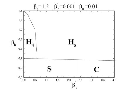
Figure 12: Mean field phase diagram in the $\beta_{g}^{\prime}-\beta_{h}$ plane for $\beta_{g}=1.2,\beta_{R}=0.01.$

It contains four phases with the following characteristics:

Quantity:	$P_{S}$	$P_{T}$	$L_{S}$	$L_{T}$	$R2$
Confining Strong Phase S:	$0$	$0$	$0$	$0$	$1$
Coulomb Phase C:	$\neq 0$	$\neq 0$	$0$	$0$	$1$
Four-dimensional Higgs Phase $H_{4}:$	$\neq 0$	$0$	$\neq 0$	$0$	$>1$
Five-dimensional Higgs Phase $H_{5}:$	$\neq 0$	$\neq 0$	$\neq 0$	$\neq 0$	$>1$

As we vary $\beta_{h}$ or $\beta_{g}^{\prime}$ we see the various quantities changing to values signaling the transition to some other phase. In general the phase diagram coincides with the one derived by Monte Carlo runs, apart from expected quantitative differences. However there are some remarks to be made. (a) The mean field method always yields a phase transition separating the $S$ and $C$ phases. The Monte Carlo simulation for $\beta_{g}=0.5$ does not exhibit a $C$ phase. It appears that this phase transition line at strong gauge coupling is present only in high-dimensional space-times, where the Mean Field approach is more reliable. Of course, if the gauge coupling is weak, the $C$ phase also exists for relatively low–dimensional space-times. (b) The phase transitions are predicted to be first order by the Mean Field approach. However it is well known that this approach is not reliable insofar as the orders of the phase transitions are concerned. (c) It should be pointed out that there exists a phase separation on the vertical axis $\beta_{g}^{\prime}=0.$ This phase boundary is just an artifact of the specific Mean Field approach that we have adopted. The problem has already been recognised before [17] and alternative mean field approaches have been devised, which avoid this unphysical behaviour. However they seem rather ad hoc. In addition this phase transition is far from reality only for very large values of $\beta_{h}$ (of order 1), while for smaller $\beta_{h}$ the phase transition is very near the real behaviour. Thus we have decided not to use these alternatives.

We may use the Mean Field approach to explore the role of the $\beta_{h}^{\prime}$ parameter. We expect that its role will be most important when the remaining parameters initially locate the system in the $H_{4}$ phase. If we start with $\beta_{h}^{\prime}=0$ and gradually increase its value, it is natural to expect that the transverse direction will communicate more and more with the space-like directions, so gradually the system will move from the $H_{4}$ to the $H_{5}$ phase. If the system lies initially in the $S$ or the $C$ phases, it is conceivable that the system will move to a Higgs phase. However, we have chosen to find the critical $\beta_{h}^{\prime}$ for each value of $\beta_{h}(\beta_{g}^{\prime})$ when $\beta_{g}^{\prime}=0.3$ $(\beta_{h}=0.5)$ and determine in this way the critical line in the $\beta_{h}-\beta_{h}^{\prime}$ plane ($\beta_{g}^{\prime}-\beta_{h}^{\prime}$ plane). The results are contained in figures 13 and 14. We see that if $\beta_{g}^{\prime}$ (or $\beta_{h}$) are large enough, the critical $\beta_{h}^{\prime}$ tends to zero, that is the system is in the $H_{5}$ phase from the beginning. In addition we see that the value $\beta_{h}^{\prime}=0.001$ that we have used throughout the paper is small enough to permit for the existence of an $H_{4}$ phase. Finally we note that we cannot detect here the phase $C_{4}$ found by the Monte Carlo approach, namely the one with small $P_{T}$ but large $L_{T}.$ This is again due to the specific structure of our Mean Field approach. In particular the link consists of products of the gauge link variable multiplied by products of the scalar field angular variables (which yield bounded contributions). Thus it is not possible to have small gauge variables on the links (yielding the small $P_{T}$) and at the same time have a large $L_{T}.$

In addition it is possible to start with $\beta_{h}^{\prime}=0$ and the remaining variables such that the system is initially in the $S$ or the $C$ phases. It turns out that increasing $\beta_{h}^{\prime}$ the system will undergo a phase transition and move to the $H_{5}$ phase. In figure 15 we have chosen $\beta_{h}=0.3,\beta_{R}=0.01,\beta_{g}=1.2$ and scanned $\beta_{h}^{\prime}$ for various values of $\beta_{g}^{\prime}.$ In other words we scanned various regions of the $S$ and $C$ phases. The result is somehow more complicated than the ones in the previous two figures. The system moves from either $S$ or $C$ to $H_{5}.$

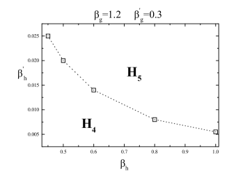
Figure 13: Phase diagram in the $\beta_{h}-\beta_{h}^{\prime}$ plane for $\beta_{g}=1.2,\beta^{\prime}_{g}=0.3,\beta_{R}=0.01.$

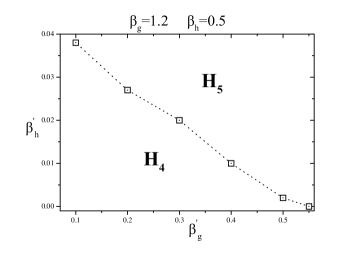
Figure 14: Phase diagram in the $\beta_{g}^{\prime}-\beta_{h}^{\prime}$ plane for $\beta_{g}=1.2,\beta_{h}=0.5,\beta_{R}=0.01.$

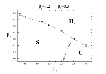
Figure 15: Phase diagram in the $\beta_{g}^{\prime}-\beta_{h}^{\prime}$ plane for $\beta_{g}=1.2,\beta_{h}=0.3,\beta_{R}=0.01.$

References

- [1] Th.Kaluza, Sitzungsber.d.Preuss.Akad.d.Wiss. (1921) 996; O.Klein, Zeitschrift f. Phys. 37 (1926) 895.
- [2] N. Arkani-Hamed, S. Dimopoulos and G. Dvali, Phys. Lett. B 429 (1998) 263, hep-th/9803315; I. Antoniadis, N. Arkani-Hamed, S. Dimopoulos and G. Dvali, Phys. Lett. 436 (1998) 257, hep-th/9804398.
-
[3]
L. Randall and R. Sundrum, Phys. Rev. Lett. 83
4690 (1999) [hep-th/9906064]; Phys. Rev. Lett. 83 3370
(1999) [hep-ph/9905221];
A. Karch and L. Randall, Int.J.Mod.Phys. A16,780 (2001) [hep-th/0011156]; A. Davidson and P.D. Mannheim, [hep-th/0009064]. -
[4]
W.D. Goldberger and M.B. Wise, Phys. Rev. Lett. 83 4922
(1999) [hep-ph/9907447]; Phys. Rev. D 60 107505 (1999) [hep-ph/9907218];
H. Davoudias, J.L. Hewett and T.G. Rizzo, Phys. Lett. B 473 43 (2000) [hep-ph/9911262];
T. Gherghetta and A. Pomarol, Nucl. Phys. B 586 141 (2000) [hep-ph/0003129];
O. DeWolfe, D.Z. Freedman, S.S. Gubser and A. Karch, Phys. Rev. D 62 0406008 (2000) [hep-th/9909134];
A. Kehagias, K. Tamvakis Phys.Lett. B 504:38-46,2001 [hep-th/0010112]; A. Kehagias, Phys. Lett. B 469 123 (1999) [hep-th/9906204]; [hep-th/9911134];
A. Pomarol, Phys. Lett. B 486 153 (2001) [hep-ph/9911294]. - [5] Y.K. Fu and H.B. Nielsen, Nucl. Phys. B 236, 167 (1984).
- [6] C.P. Korthals-Altes, S. Nicolis and J. Prades, Phys. Lett. B 316 339 (1993) [hep-lat/9306017]; A. Hulsebos, C.P. Korthals-Altes and S. Nicolis, Nucl. Phys. B 450 437 (1995) [hep-th/9406003].
- [7] P. Dimopoulos, K. Farakos, A. Kehagias, G. Koutsoumbas Lattice Evidence for Gauge Field Localization on a Brane [hep-th/0007079] (to appear in Nucl. Phys. B); P. Dimopoulos, K. Farakos, G. Koutsoumbas, C.P. Korthals-Altes, S. Nicolis, J. High Energy Phys. 02(005) (2001) [hep-lat/0012028]; P. Dimopoulos, K. Farakos, S. Nicolis, Multilayer Strucure in the Strongly Coupled 5-D Abelian Higgs Model, [hep-lat/0105014]
- [8] D. Berman and E. Rabinovici, Phys. Lett. 157 B 292 (1985).
-
[9]
Guo-Li Wang and Ying-Kai Fu [hep-th/0101146];
Liang-Xin Huang, Ying-Kai Fu and Tian-Lun Chen, J.Phys. G 21 1183 (1995). - [10] S. Ejiri, J. Kubo and M. Murata, Phys. Rev. D 62 105025 (2000), [hep-ph/0006217].
- [11] S. Nadkarni, Nucl. Phys. B 334, 559, (1990); A. Hart, O. Philipsen, J.D. Stack and M. Teper, Phys. Lett. B 396, 217 (1997) [hep-lat/9612021].
- [12] V.K. Mitrjushkin and A.M. Zadorozhny, Phys. Lett. B 181 111 (1986).
- [13] A.T. Barnaveli and O.V. Kancheli, Sov. J. Nucl. Phys. 51(3) (1990).
- [14] G. Dvali and M. Shifman, Phys. Lett. B 396, 64 (1997) ; Erratum-ibid. B 407, 452 (1997) [hep-th/9612128].
- [15] M. Creutz, Phys. Rev. Lett. 43 553 (1979); Phys. Rev. D 21, 2308, (1980).
- [16] H. Kawai, M. Nio and Y. Okamoto, Prog. Theor. Phys. 88, 341 (1992).
- [17] R. Baier and H.-J. Reusch, Nucl. Phys. B 285[FS19] (1987) 535.
- [18] Y.K. Fu and H.B. Nielsen, Nucl. Phys. B 254 (1985) 127.