Analytic calculation of the mass gap in U$(1)_{2+1}$ lattice gauge theory.

Abstract

An analytic calculation of the photon mass gap $M$ of compact U$(1)_{2+1}$ in the Hamiltonian formalism is performed utilizing the first four Hamiltonian moments with respect to a one-plaquette mean field state in the plaquette expansion method. Scaling of $M$ is clearly evident at and beyond the transition from strong to weak coupling. The scaling behaviour agrees well with the range of results from numerical calculations.

1 Introduction

In QCD, the most fundamental quantities one wishes to calculate are the states of the mass spectrum of the theory. In lattice gauge theory, such non-perturbative calculations are carried out numerically in the path integral representation to some level of approximation by evaluating the correlation functions by Monte-Carlo simulation. Typically, the computational resources employed in this approach are enormous as one must work with large lattices and spacings which are fine enough to detect the continuum behaviour of the theory in question. Hence, non-perturbative analytic results are of considerable interest. In this context, the Hamiltonian formalism is appealing. One often works directly on infinite lattices, fermions are simpler to incorporate (no fermion determinant) and 3D as opposed to 4D lattices (time is continuous). The lack of systematic and applicable methodology has prevented these features from being exploited or investigated - hence, the importance of new methodologies. Here we use a novel approach – the plaquette expansion – based on a large volume expansion of Lanczos tridiagonalization.

2 Compact U(1) in 2+1 Dimensions

Compact U$(1)_{2+1}$ has become the testing ground for various lattice Hamiltonian procedures as it exhibits scaling behaviour similar to the more complex and physically interesting non-abelian lattice gauge theories in $3+1$ dimensions. The Kogut-Susskind Hamiltonian is [2]:

$$H=\frac{g^{2}}{2}\sum_{l}{\hat{E}}^{2}_{l}+\frac{1}{2g^{2}}\sum_{p}\left[2-({\hat{U}}_{p}+{\hat{U}}_{p}^{{\dagger}})\right]\ ,$$ (1)

where $g$ is the dimensionless coupling constant. The strong-coupling limit is defined by $g\rightarrow\infty$ and the weak-coupling limit by $g\rightarrow 0$. The electric field operator, ${\hat{E}}_{l}$, and link operator, ${\hat{U}}_{l}$ obey the commutator relations $[{\hat{E}}_{l},{\hat{U}}_{l}]={\hat{U}}_{l}$ and $[{\hat{E}}_{l},{\hat{U}}_{l}^{{\dagger}}]=-{\hat{U}}_{l}^{{\dagger}}$ and the plaquette operator ${\hat{U}}_{p}$ acts on the links around the smallest closed (Wilson) loop or square on the lattice ${\hat{U}}_{p}={\hat{U}}_{1}{\hat{U}}_{2}{\hat{U}}_{3}^{{\dagger}}{\hat{U}}_{4}^{{\dagger}}$.

One of the quantities of interest in this model is the anti-symmetric or photon mass gap, $M$ ( $\equiv M_{0^{+-}}$ ), which is given by the difference in energies between the lowest state in the $0^{+-}$ sector and the vacuum. The scaling behaviour for the mass gap is expected to be [1]: $M^{2}a^{2}\equiv\beta\mbox{exp}\{-k_{0}\beta\ +\ k_{1}\}$, where $k_{0}$ and $k_{1}$ are constants, $a$ is the lattice spacing and $\beta=1/g^{2}$. The scaling parameters $k_{0}$ and $k_{1}$ are not known exactly but have been computed by various numerical techniques: $k_{0}\sim 4.1-6.345$ and $k_{1}\sim 4.369-6.27$ (See [3] for summary).

3 Plaquette Expansion

Beginning with a trial state $|\psi_{1}\rangle$ which has the desired symmetries of the state of interest, the Lanczos recurrence generates a basis

$$|\psi_{n}\rangle=\frac{1}{\beta_{n-1}}\left[\left(H-\alpha_{n-1}\right)|\psi_{n-1}\rangle-\beta_{n-2}|\psi_{n-2}\rangle\right],$$

where $\alpha_{n}=\langle\psi_{n}|H|\psi_{n}\rangle$ and $\beta_{n}=\langle\psi_{n+1}|H|\psi_{n}\rangle$ are the matrix elements of the Hamiltonian in tri-diagonal form.

The matrix elements are able to be written in terms of Hamiltonian moments $\langle H^{n}\rangle\equiv\langle\psi_{1}|H^{n}|\psi_{1}\rangle$. The connected part of the Hamiltonian moment is proportional to the volume of the system $\langle H^{n}\rangle_{c}=e_{n}\,N$. Therefore, one may re-express the matrix elements in terms of the connected vacuum coefficients $e_{n}$. Extensivity of the problem leads to the following plaquette expansions in $1/N$ [4]:

$${\alpha_{n}\over N}=e_{1}+s\left[\frac{e_{3}}{e_{2}}\right]+O(s^{2})\equiv{\bar{\alpha}}(s),$$ (2)

$${\beta_{n}^{2}\over N^{2}}=se_{2}+\frac{1}{2}s^{2}\left[\frac{e_{2}e_{4}-e^{2}_{3}}{e^{2}_{2}}\right]+O(s^{3})\equiv{\bar{\beta}^{2}(s)}$$ (3)

where $s\equiv n/N$. In the bulk limit ($n,N\rightarrow\infty$), keeping $s$ fixed, one may perform the exact diagonalization of the Lanczos tri-diagonal matrix for the ground state energy density $\varepsilon_{0}$ analytically [5]: $\varepsilon_{0}={\rm inf}\,({\bar{\alpha}}(s)-2{\bar{\beta}(s)})\,$. For example, for 4th order moments we have:

$$\varepsilon_{0}[4]=e_{1}+\frac{e_{2}^{2}}{e_{2}e_{4}-e_{3}^{2}}\,\left[\sqrt{3e_{3}^{2}-2e_{2}e_{4}}-e_{3}\right].$$ (4)

For excited states the Hamiltonian moments have the form $\langle H^{n}\rangle^{(S)}_{c}=e_{n}N+m_{n}^{(S)}$. Thus, in a similar fashion to $\varepsilon_{0}$, one can derive expressions for approximants, $M^{(S)}_{0}[r]$, to the mass gap. Again using up to 4th order moments we have [6]:

$$M^{(S)}_{0}[4]=\sum^{4}_{n=1}\,m^{(s)}_{n}\,e_{2}^{n-1}\,F_{n}(e_{2},e_{3},e_{4}),$$ (5)

where the vacuum moment functions, $F_{n}$, are simple algebraic forms given in [6].

4 One Plaquette Mean-Field State

Initially, lattice Hamiltonian calculations employed the simplest gauge invariant trial state — the strong-coupling vacuum $|0\rangle$ (defined as the state satisfying ${\hat{E}}_{l}|0\rangle=0$ for every link). This is the perturbative starting point for series calculations, which are then extrapolated to weak coupling. Although the calculation of moments with respect to this state can be carried out to relatively high order, typically, one finds that this state is simply inadequate to explore the non-perturbative weak-coupling regime of the theory. In the case of the plaquette expansion, a window of scaling in terms of the expansion order was evident, but higher order results became problematic [7].

                 

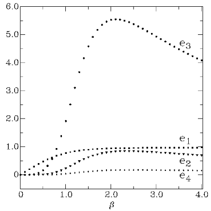
Figure 1: Ground state moments, $e_{1}\rightarrow e_{4}$.

Here we utilized a one plaquette exponential trial state, that has the correct strong and weak coupling behaviour for the vacuum energy density – the so-called mean-field state [8] – defined in the so-called $U$ representation as:

$$\psi_{1}[U_{p}]=\exp\left\{\frac{\lambda}{2}\sum_{p}\left\{{U}_{p}+{U}_{p}^{\dagger}\right\}\right\}$$ (6)

where $\lambda$ is determined variationally from $\langle H\rangle$. As the state is constructed from plaquette variables, $U_{p}$, it is automatically gauge invariant. One expects the true ground state of the system to have contributions from all possible Wilson loops – an important feature of the plaquette expansion method is that, by its very nature, larger sized Wilson loops (larger clusters) are systematically introduced.

Using a diagrammatic method (details to be presented elsewhere) we were able to derive the first four one-plaquette connected moments for both the ground state and anti-symmetric state. The expressions become rather long, so for brevity these are illustrated in Figures 1 and 2, along the curve $\lambda(\beta)$. These moments immediately give analytic approximates for vacuum energy and the mass gap.

                 

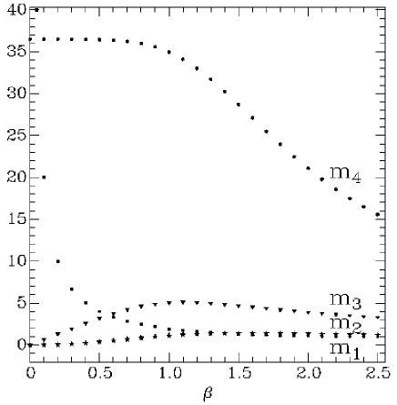
Figure 2: Anti-symmetric moments, $m_{1}\rightarrow m_{4}$.

5 Results and Discussion

The plaquette expansion results are presented in Figure 3. Clearly scaling is evident for inverse-coupling values $\beta=0.7$ to $1.5$, passing the transition point at $\beta=1.0$. The scaling form we find is given by $M^{2}=\beta\,\mbox{exp}\left(-4.34\beta+5.34\right)$, and agrees well with other estimates (summarized in [3]).

         

Figure 3: Mass gap results applying one, three and four one-plaquette Hamiltonian moments. Scaling is evident for the four order moments curve from $\beta=0.7$ to $1.5$.

Although we have presented results for only the first four moments (for which the calculation is entirely analytic) it should in principle be possible to derive higher moments with respect to this state. Indeed we have preliminary results for the ground state energy density to sixth order giving high accuracy over a large range of couplings.

For the future application of this method to $\mbox{QCD}_{3+1}$, the main obstacle to overcome is the calculation of the moments in 3+1 dimensions. The appeal of 2+1 systems as toy models is that the transformation from link variables to plaquette variables is trivial and makes the integrations tractable – hence the analytic work reported here. In 3+1 dimensions it is well known that the transformation cannot be carried out in closed form due to the appearance of Bianchi identities. However, the calculation of moments in 3+1 dimensions by Monte-Carlo is actually a relatively small scale numerical exercise. Because we are dealing with a cluster expansion (we need only connected moments) the lattices required are fairly modest in extent and, by definition, only 3 dimensional. The integrands become complicated as larger correlations are included, which means that the statistics must be very good, however, preliminary calculations have demonstrated that the required precision is possible to achieve without supercomputing resources.

References

- [1] M.Gpfert and G.Mack, Commum. Math. Phys. 82, 545 (1982).
- [2] J.Kogut and L.Susskind, Phys. Rev. D 11, 395 (1975).
- [3] J.A.L.McIntosh, Ph.D. thesis, University of Melbourne (2000).
- [4] L.C.L.Hollenberg, Phys. Rev. D 47, 1640 (1993).
- [5] L.C.L.Hollenberg and N.S.Witte, Phys. Rev. B 54, 16309 (1996).
- [6] L.C.L.Hollenberg, M.Wilson and N.S.Witte, Phys. Lett. B 361, 81 (1995).
- [7] J.A.L.McIntosh and L.C.L.Hollenberg, Z. Phys. C 76, 175 (1997).
- [8] S.J.Baker, R.F.Bishop and N.J.Davidson, Phys. Rev. D 53, 2610 (1996).